👀 계량경제학 개인 공부용 포스트 글 입니다.
Ch7. Nonlinear relationship
① Polynomials
• Polynomials are useful to capture relationships that are curved.
⇨ examples
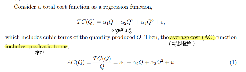
(1) Cost functions
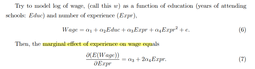
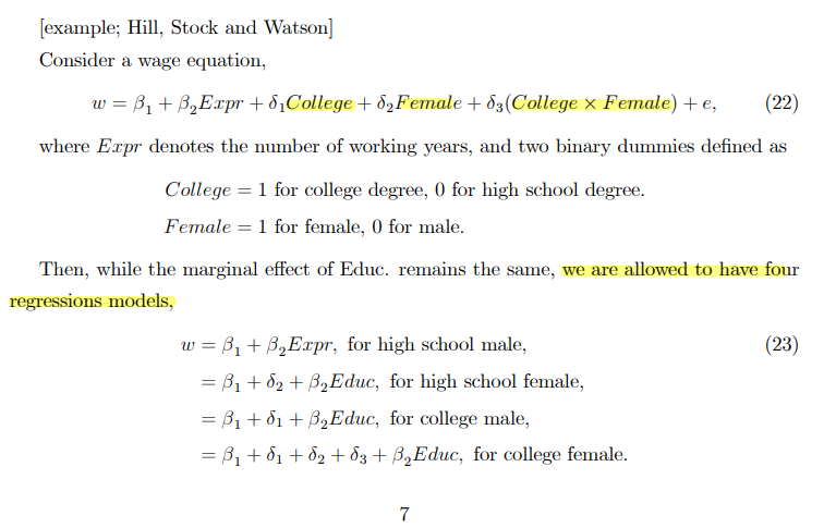
(2) Wage function
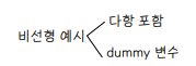
② Nonlinear relations
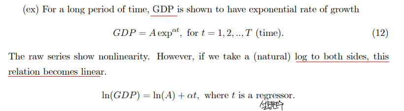
• GDP 는 exponential 한 추이를 보인다. 그러나 log 를 씌우면 linear 한 관계를 보일 수 있다.
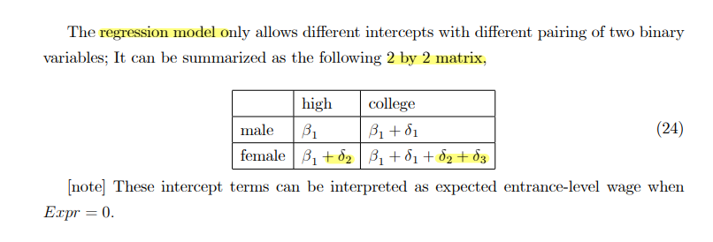
③ Use of Dummy variables
• nonlinear 한 관계를 만드는 가장 간단한 방법은 dummy (binary) 변수를 찾는 것이다.

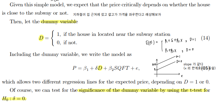
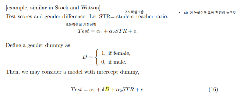
• Intercept dummy : 절편에 영향을 주는 더미변수
• Slope dummy : 기울기에 영향을 주는 더미변수
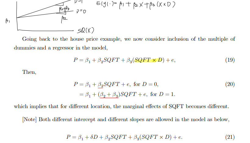
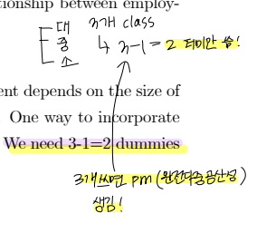
• Interacting dummies : 더미변수의 교차항
Ch8. Heteroskedasticity: Unequal variance
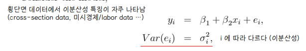
① Nature of Heteroskedasticity
• simple linear regression model 을 고려했을 때, Var(ei) = σ^2 등분산성 가정을 도입했었다. 이번에는 i 마다 분산이 다른 경우 (이분산성) 를 살펴보자
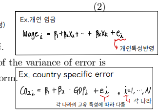
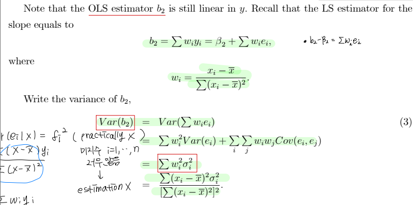
② OLS estimator under 이분산성
• 정의와 예시
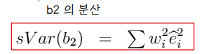
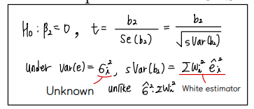
• 이분산성이 있을 때, b2 추정하기
③ Generalized LS estimator
• variance of errors can be different for different observations
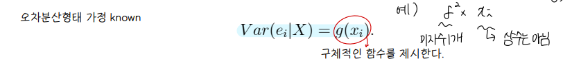
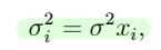
• 복잡성을 줄이는 방법은, 아래와 같이 분산을 x 값에 의존하는 어떠한 함수로 구성하는 것이다.
• 이분산성 error 에 대한 구체적인 형태를 가정하기 위해, 가장 best 인 LS estimator 를 살펴본다 ⇨ GLS
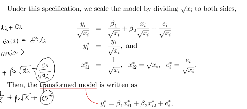
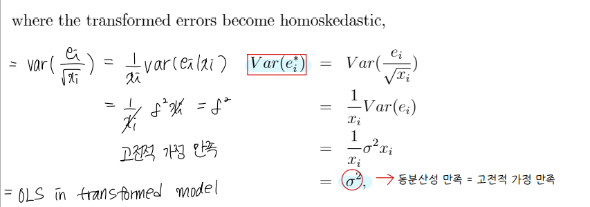
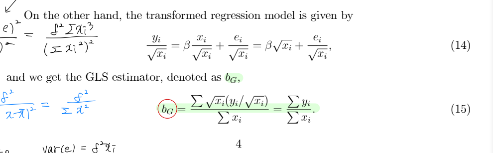
• Transforming the model
• Efficiency of GLS estimator : GLS 가 OLS 보다 효율적이다 = more efficient = GLS 의 분산이 더 작다
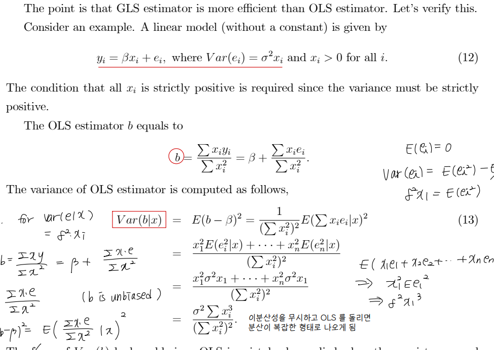
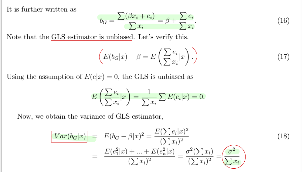
⇨ Var(bG) < Var(b) : GLS more efficient than OLS
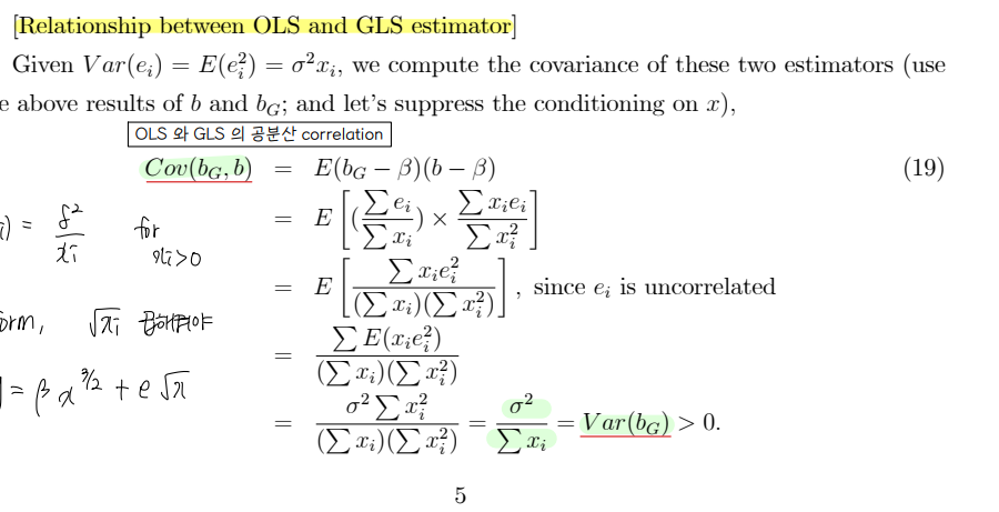
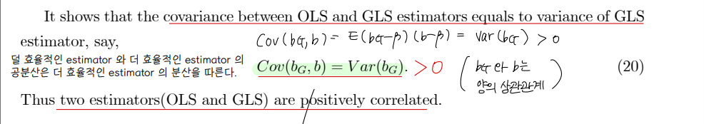
• OLS 와 GLS 추정치의 관계
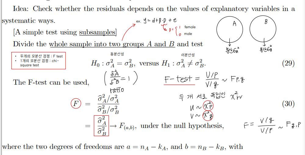
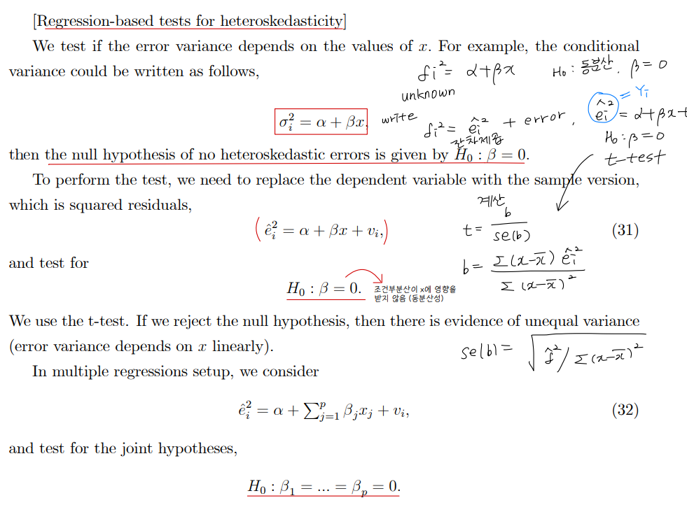
④ Testing for Heteroskedasticity
• 이분산성 검정
Ch9. Dynamic models, Autocorrelation, and forecasting
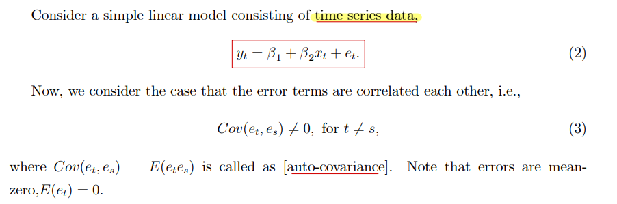
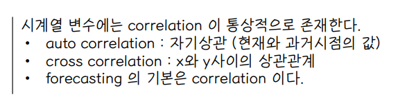
① Autocorrelation
• 자기상관 : x_t, x_t-1
• correlations of errors between the two different time points, denoted as autocorrelation.
• error term 에서 자기상관성이 관찰된 상황을 살펴보자 ⇨ error 사이에는 상관관계가 없다는 고전적 가정 위배
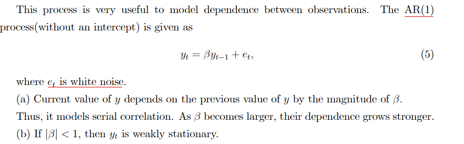
• Popular model for autocorrelation ⇨ AutoRegressive progress
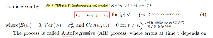
⇨ AR(1) 에서의 가정 : |ρ| < 1
⇨ ρ는 et 가 e_t-1 에 의존하는 정도를 결정한다.
⇨ ρ 값이 크다면, 현재 값이 이전 값에 강하게 의존한다는 의미
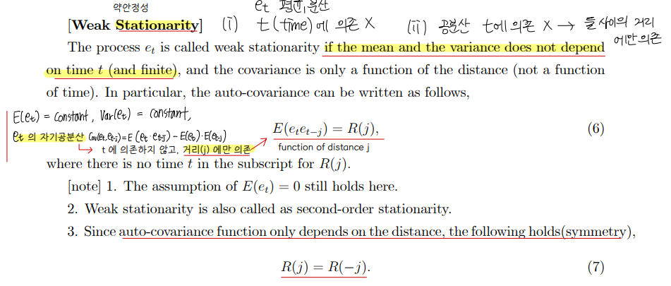
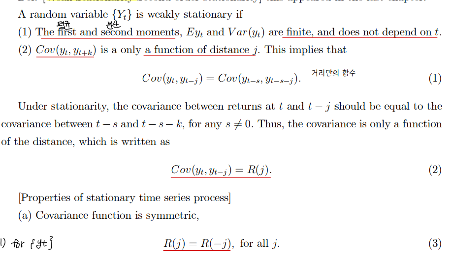
• Weak Stationarity : 평균과 분산이 t 에 의존하지 않는 경우
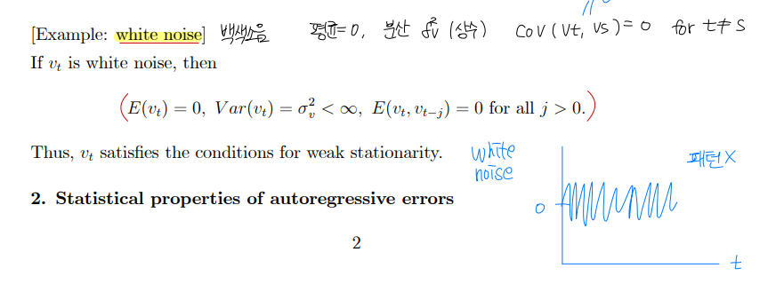
• White noise
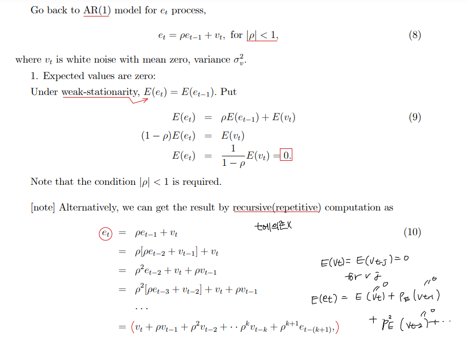
② Statistical properties of autoregressive errors
• et 는 recursive 한 term 으로 작성해볼 수 있따.
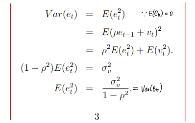
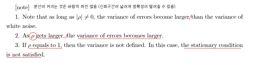
• variance of errors
• Note
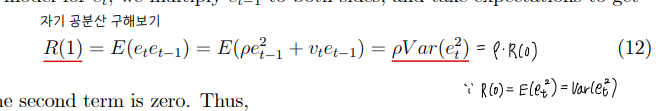
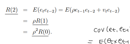
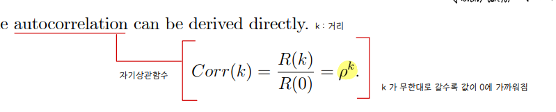
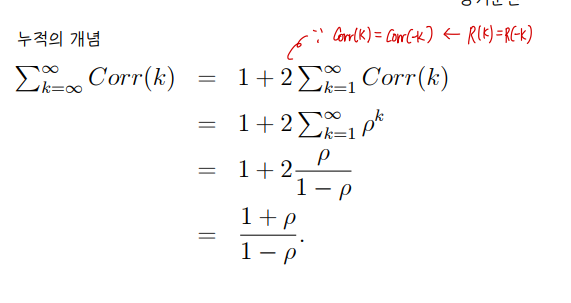
③ Covariance and correlation function of errors
• 자기공분산
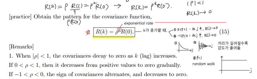
• autocorrelation
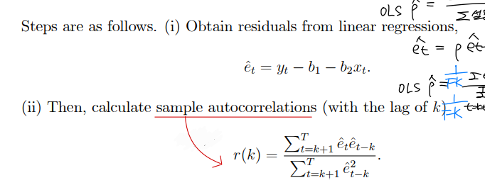
④ Computing sample autocorrelations
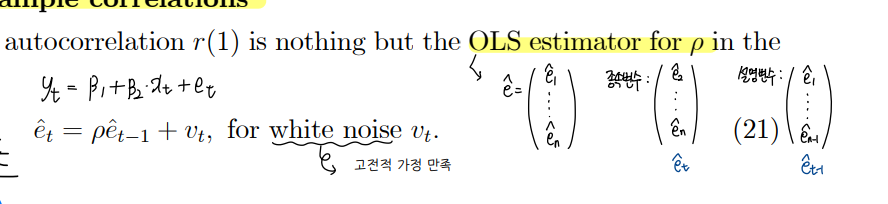
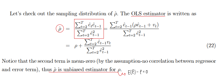
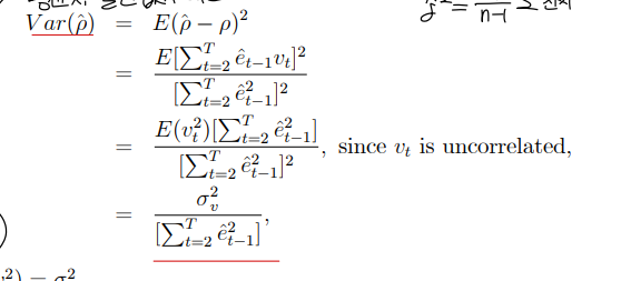
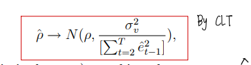
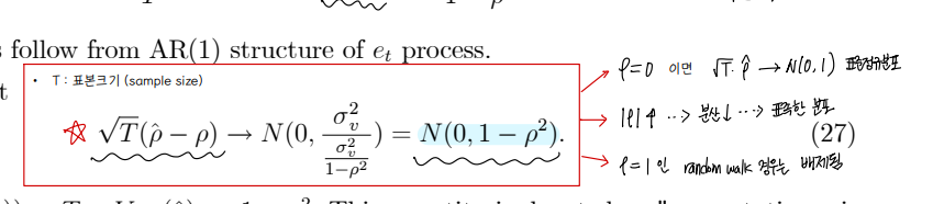
⑤ Distribution of sample correlations
• ρ estimation
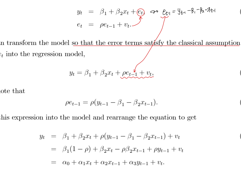
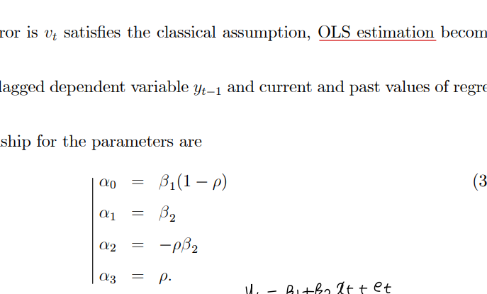
⑥ Estimating a linear model with correlated errors
• Transformation
⑦ Testing for autocorrelation
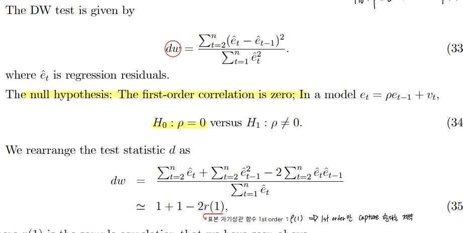
• Testing for 1-lag correlation: Durbin-Watson (DW) test
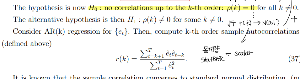
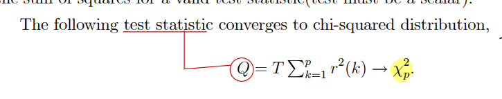
• Testing for k-lag correlation : Box and Pierce Test
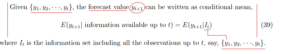
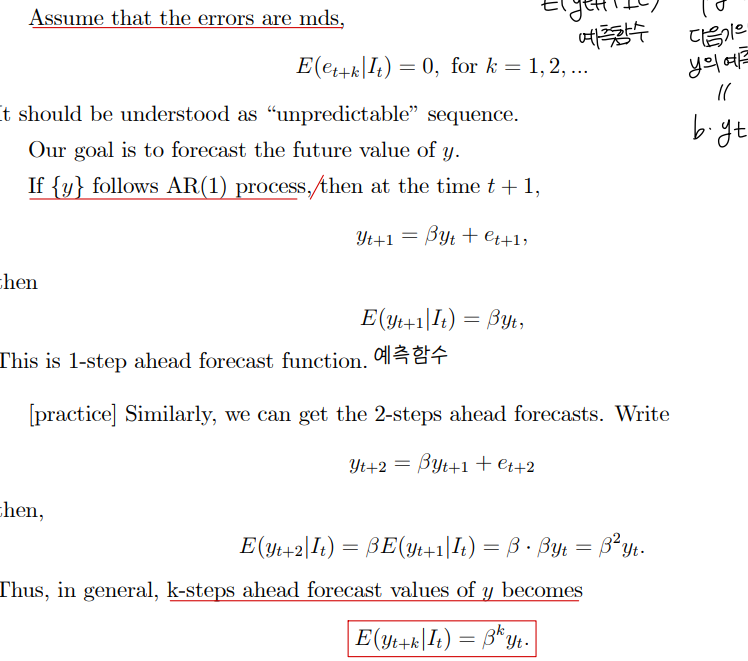
⑧ Simple forecasting
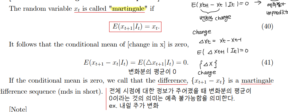
• Martingale difference sequence
• Simple forecasting based on AR(1) model
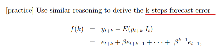
• Forecast error

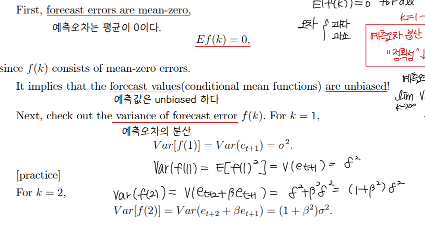
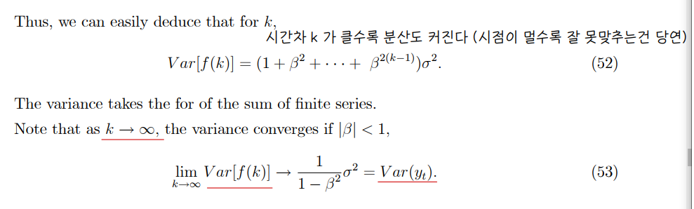
• Properties of forecast error
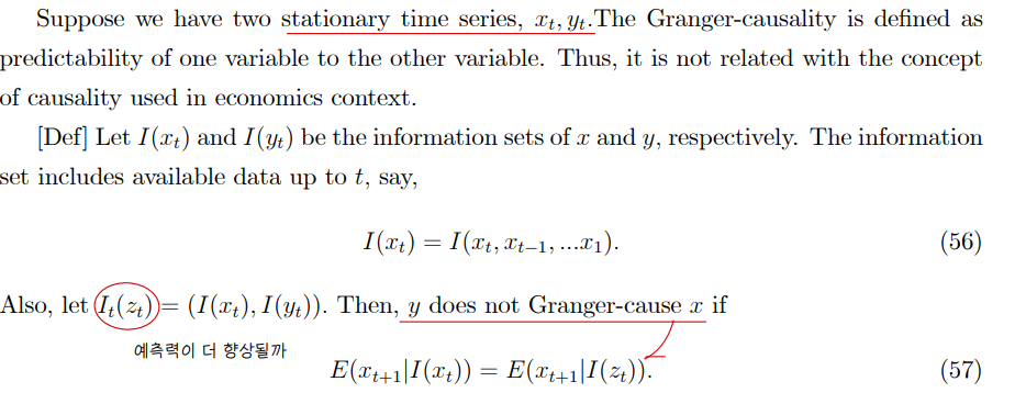
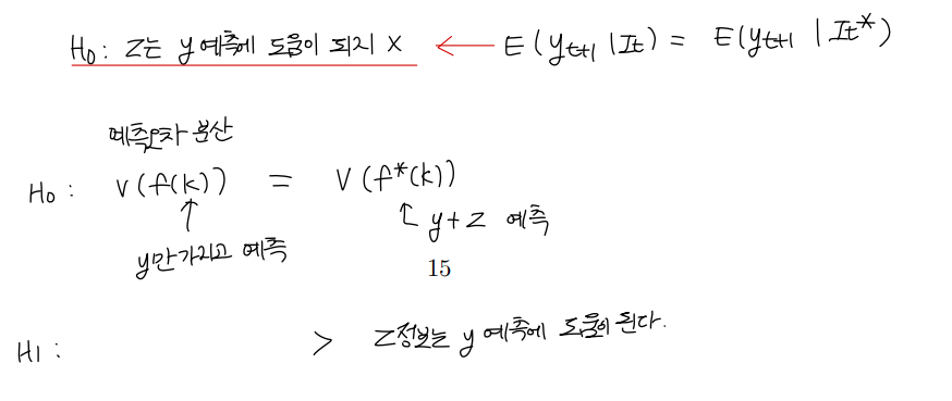
⑨ Granger-Causality- application of forecasting
• xt, yt 의 2개의 정상 시계열이 있다고 가정하자. 이 두 시계열의 정보가 함께 주어졌을 때, x_t+1 을 예측한다고 하면, 예측력이 더 향상될까
Ch10. Introduction to Time series
① Properties of Time Series
• time series econometrics at a basic level
• time series data
- High frequency data : Intervals of observations are short-financial data (daily data)
- low frequency data : Intervals are long, i.e., quarterly, or annual data mostly, macroeconomic data
• Weak stationarity 정상성
• Autoregressive process
• Random Walk process
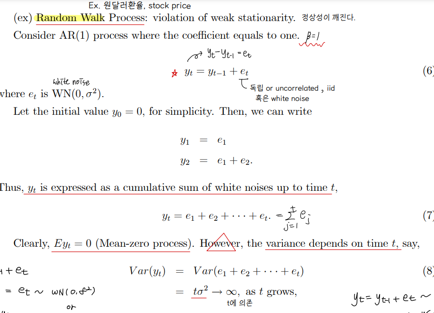
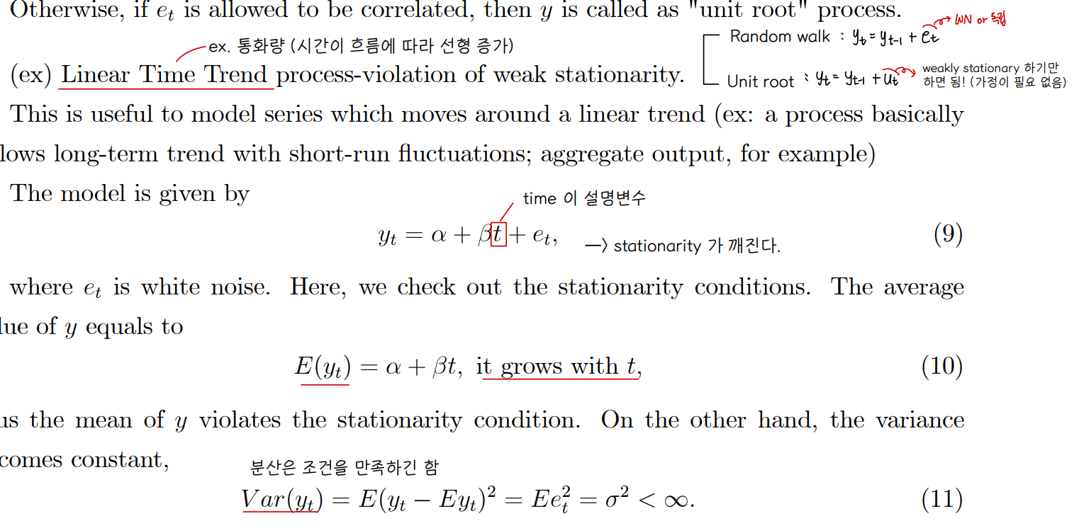
• Unit root process
② Models for stationary time series
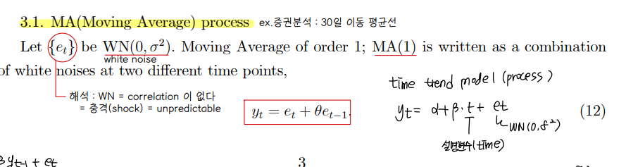
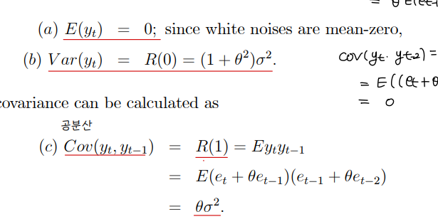
• Moving average process , MA(1)
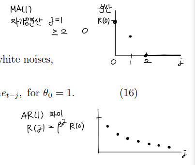
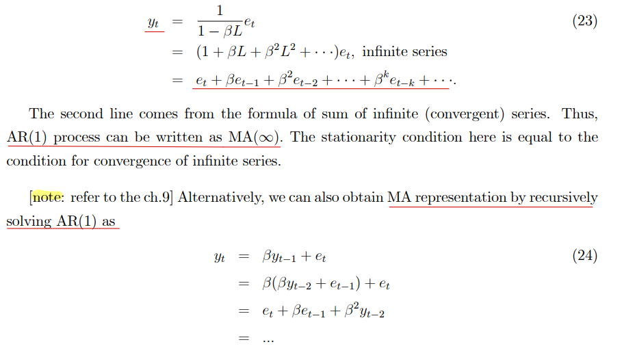
• MA representation of AR(1) process
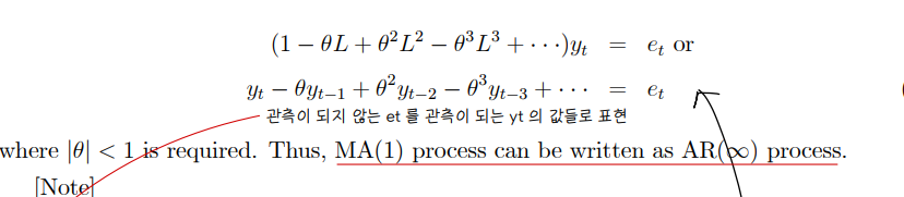
• AR representation of MA(1) process
• ARMA

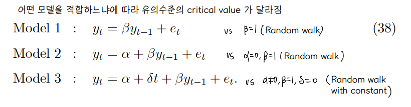
③ Testing for unit root
• 단위근 검정 (=stationarity testing) : 단위근이 있다면 non-stationary 한 시계열

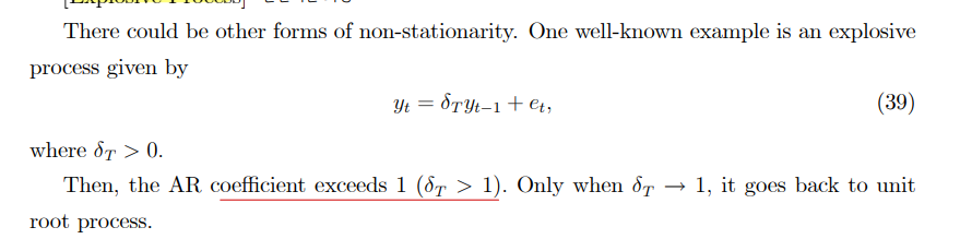
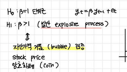
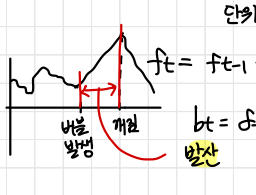
• Explosive process 발산하는 과정
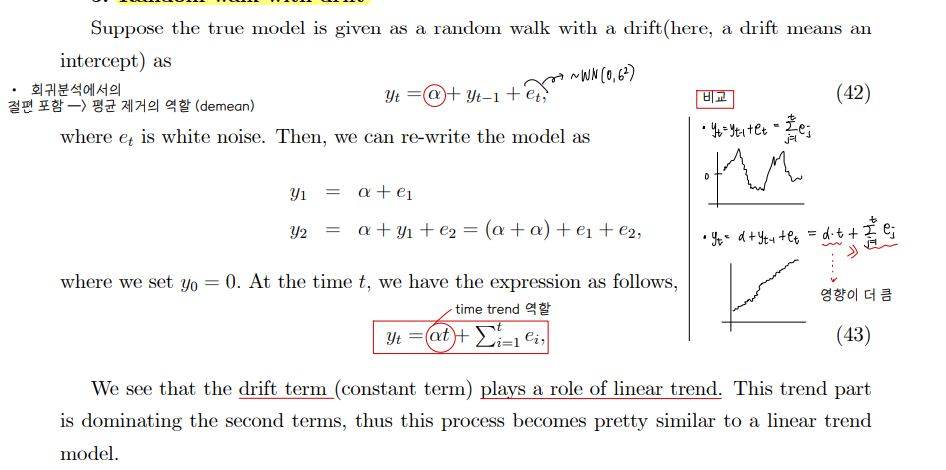
④ Random walk with drift
• drift = intercept
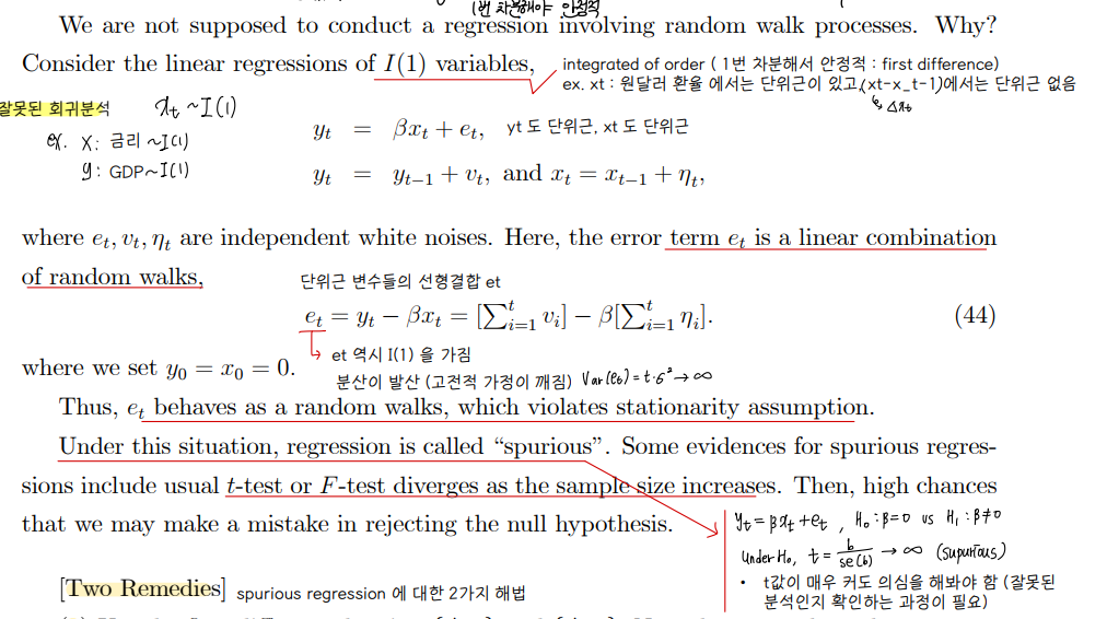
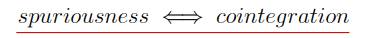
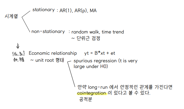
• Spurious regression (misleading regression)
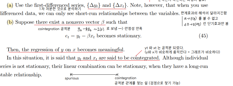
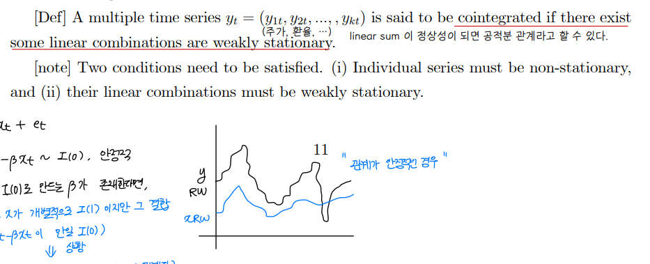
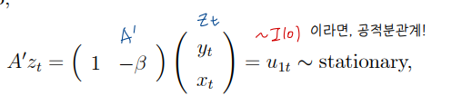
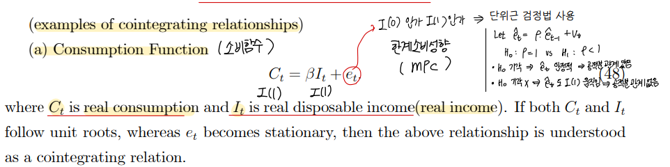
⑤ Cointegrations
• linear sum 이 정상성이 되면 공적분 관계라고 할 수 있다.
• 변수가 공적분 관계라는 것은 안정적인 관계가 형성된 것이라고 해석해 볼 수 있다. 공적분 관계가 성립하면 검정이나 추정들이 유효해진다.
• 변수가 3개면 가능한 공적분의 개수는 2이다.
• 공적분 관계
• Spuriousness 와 cointegration 은 상반된 관계
• Ex. 공적분 관계 : Consumption function 소비함수
✏ summary
'1️⃣ AI•DS > ⚾ 계량경제•통계' 카테고리의 다른 글
| 계량경제학 스터디 CH11,12,13,14,15정리 (0) | 2023.04.09 |
|---|---|
| Difference-in-Difference (DiD) (0) | 2023.04.03 |
| 계량경제학 스터디 CH3,4,5,6 정리 (0) | 2023.03.19 |
| 계량경제학 스터디 CH1,2 정리 (1) | 2023.03.13 |
| Introduction to statistical learning - ch2 (0) | 2022.08.02 |


댓글