👀 Keyword
◯ Quasi-experimental research design
• DiD
• DDD
• Probit model
• Hazard model
◯ Matching
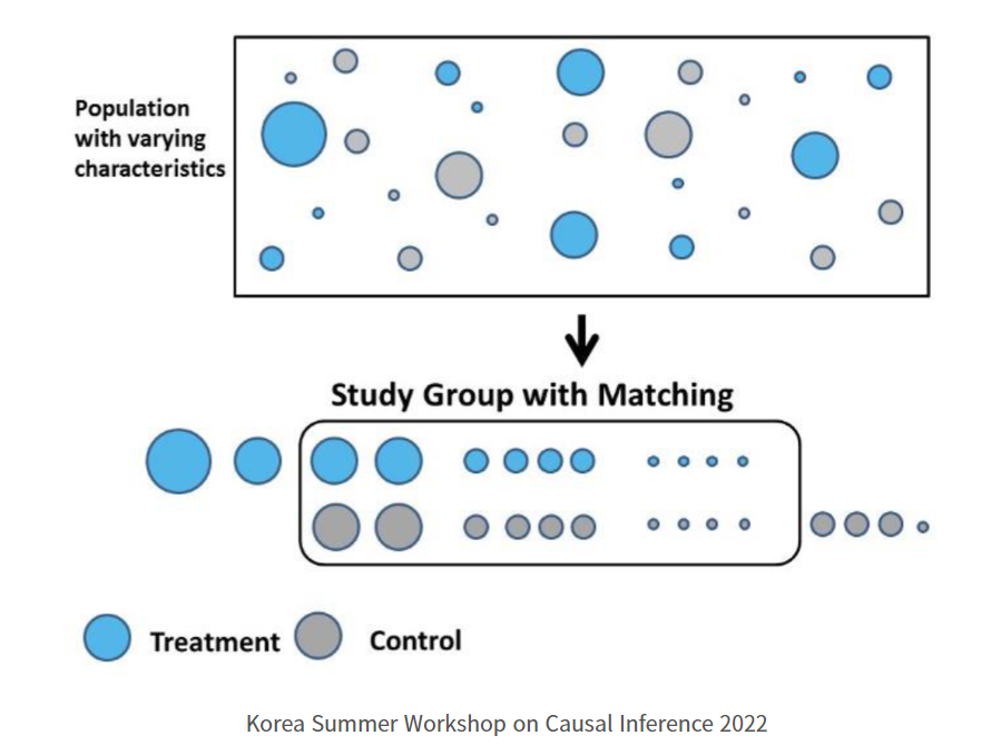
• CEM : 단순하게 통제변수들이 비슷한 관측치끼리 매칭하는 방법

• PSM : 통제 변수가 주어진 상태에서 Treatment 를 받을 확률 (Propensity score) 이 비슷한 관측치끼리 매칭

• EDM : 유클리디안 거리를 기준으로 매칭
👀 데이터 해석을 위한 도메인 지식
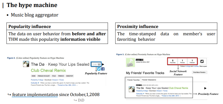
◯ The hype machine
• Largest MP3 blog aggregator 로 블로그에 포스팅 된 음악/트랙 리스트들을 수집하여 관련 정보를 제공한다. 유저들은 음악을 스트리밍 할 수 잇으며, 음악 다운로드는 불가능하다.
• 연구를 진행한 시점에서 15~20% 에 해당하는 유저들만 social networking 기능들을 사용하고 있었고 나머지 유저들은 isolate (다른 유저들을 팔로우 하지 않음) 되어 있었다.
• Popularity information 은 웹사이트의 모든 유저들에게 10월 1일을 기점으로 모두에게 보여졌다. 10월 1일 시점 이전에도 유저들은 좋아요를 누를 수 있었다. (favorites 숫자는 볼 수 없었음)
• 유저들에게 social network 를 생성할 수 있는 개별적인 대시보드를 제공하는데, 좋아하는 트랙이나 유저를 추가할 수 있다. (add favorite tracks and favorite users) 유저를 favorite 하는 것은 following 과 비슷한 행동이다. (일방향 팔로우도 가능)
① Abstract
◯ Research Topic
• 온라인 음악 커뮤니티에서 발생하는 음악 소비에 있어 Popularity influence (대중성) 와 Proximity influence (근접성) 가 미치는 영향
◯ Research Question
• RQ1. How does popularity influence affect music consumption choices?
• RQ2. Is popularity influence more important for mainstream or niche music?
• RQ3. How important is proximity influence on music consumption?
• RQ4. What is the nature of the interaction between the two types of influence? Are they complements or substitutes?
◯ Research Method
• quasi-experimental research design
• highly granular data from an online music community
◯ Research Results
• Popularity influence 와 Proximity influence 모두 음악소비에 Positive 한 영향을 끼침을 증명
• 두 영향은 서로 substitute 관계를 가지고 있으며, Proximity 영향이 있는 경우 Popularity 영향을 뛰어 넘는 것으로 나타났다.
◯ Research Contribution
• Design and marketing strategies for online communities
② Introduction
◯ Preliminary
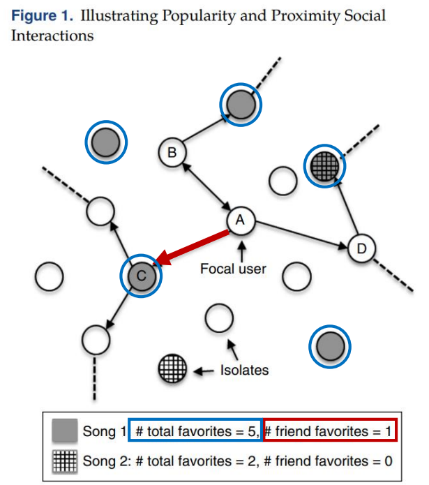
• Total favorites → Popularity influence, Friend favorites → Proximity influence
• ex. A 유저가 중심 유저에 해당할 때, Song1 의 경우 총 5명의 유저들이 좋아하고, A유저와 친구를 맺고있는 유저 중에는 C만 좋아요를 눌렀다. Song2 의 경우 총 2명의 유저가 좋아하고, A유저와 친구인 유저들 중에는 해당 노래를 좋아요를 누른 사람이 없다.
◯ Research Design

• Popularity influence → 유저의 좋아요 행동 집계를 "보이게 한 기능" (총 좋아요 수가 보이는지 여부) 을 대상으로 하여 분석을 진행 : CEM matching and DiD
• Proximity influence → 팔로우한 친구의 특정 노래에 대한 좋아요를 누른 행동 (focal user 가 좋아하는 노래를 주변 친구들도 좋아하고 있는지 여부) 을 대상으로 분석을 진행 : PSM or EDM matching and Probit model, Hazard model
③ Literature Review
◯ Popularity influence
• Online Word of mouth (Mizerski 1982, Chevalier and Mayzlin 2006, Liu 2006)
• Observational learning (Sorenson 2007, Duan et al. 2009, Salganik et al. 2006)
⇨ In study, the number of favorites for a song is hybrid of WOM and OL
◯ Proximity influence
• Influence in social networks (Brown et al. 1987, Valente 1995, Katz et.al 1955, Granovetter 1973)
• Separating social influence and homophily : Aral et al.2009 (Dynamic matched sample estimation) ⭐
④ Methodology
◯ Data
• The hype machine 이라는 음악 커뮤니티에서 데이터를 수집
• Popularity influence : Feature implementation (좋아요 수를 보이게 한 기능) 을 도입한 시점 전후를 기준으로, Song level 에서 특정 음악에 대한 총 청취 횟수를 추적
• Proximity influence : User-song level 에서 특정 유저를 기준으로 특정 음악에 대해, 주변 친구들도 좋아요를 눌렀는지 여부를 기준으로 음악 청취 여부를 추적
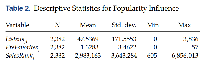
• Descriptive statistics
◯ Variable
• Popularity influence → DiD (Song level)
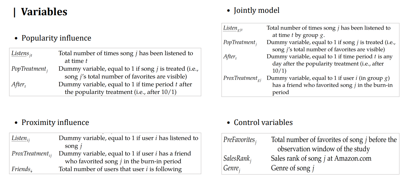
↪ Listens_jt : song j 에 대한 time t 시점의 총 청취 횟수
↪ PopTreatment_j : song j 에 대한 총 좋아요 개수가 보이는지에 대한 여부
↪ After_t : popularity treatment 이후 시점인지에 대한 여부 (총 좋아요 개수가 보이는 기능 도입 시점 이후)
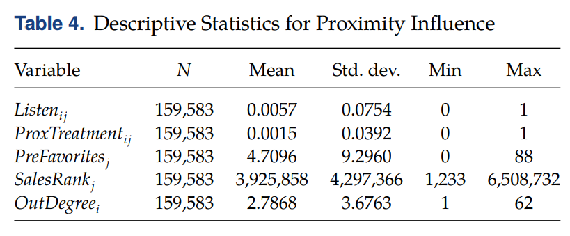
• Proximity influence (User-song level)
↪ Listen_ij : 유저 i 이 song j 를 들었는지 여부
↪ ProxTreatment_ij : 유저 i 의 팔로우 친구 중에 song j 에 대해 좋아요를 누른 친구가 있는지 여부 (0이면 좋아요를 누른 친구가 한 명도 없다는 것을 뜻함)
↪ Friends_i : 유저 i 가 팔로우하고 있는 총 유저의 수
• Jointly model → DDD (User-song granularity level)
↪ Listen_gjt : group g (주변에 해당 음악을 좋아하는 친구가 있는지 여부를 기준으로 집단을 구분) 에 대해 t 시점에 song j 를 청취한 총 횟수 👉 Popularity 와 Proximity 를 동시에 고려
※ g : index of proximity treatment (0 or 1)
⇨ g = 1 이면 ProxTreatment = 1, g=0 이면 ProxTreatment = 0
↪ PopTreatment_j : song j 에 대한 popularity influence treated 여부 (좋아요 수 보이는 기능 적용여부)
↪ After_t : 10월 1일 이후면 1, 아니면 0
↪ ProxTreatment_gj : group g 에 속하는 유저 i 가 song j 에 대해 좋아요를 누른 친구가 있다면 1, 아니면 0
• Control variable
↪ PreFavorites_j : song j 에 대해 연구 관측 시점 이전에 받았던 총 좋아요 개수
↪ SalesRank_j : 아마존에 올라온 song j 의 총 판매 순위
↪ Genre_j : song j 의 장르
◯ Model
⑴ Popularity influence
▢ CEM
• Match the two groups of songs (매칭 단위 : Song, e.g. Song A - Song B)
• 매칭 기준 : 장르, feature implementation 이전 시점의 총 좋아요 개수, 아마존 음반 판매 순위 등 관측 가능한 특성들을 기준으로 매칭을 진행
• 장르는 정확히 매칭시키도록 했고, 연속변수에 해당하는 변수들은 최대한 근접한 값을 가지도록 매칭했다. (Stata 툴 사용)
• 매칭을 통해 treatment group 과 control group 에 있는 imbalance 가 감소함을 확인
▢ DiD setting
• Assumption : 좋아요 수를 보이게 한 popularity influence 가, 음악 소비에 Positive 한 영향을 미칠 것이라고 가정 (ATE)
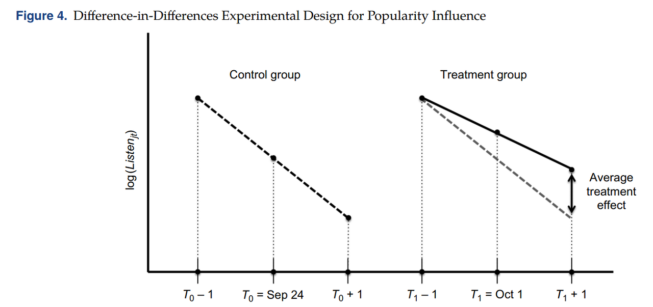
○ PopTreatment_j
• Treatment group : 좋아요 수를 "보일 수 있게 하는" 기능을 도입한 시점이 10월 1일이기 때문에, 좋아요 수가 어느정도 쌓일 수 있도록 2008년 9월 29일에 포스팅된 song 들을 기준으로 data set 을 구성
• Control group : 좋아요 수를 "보일 수 있게 하는" 기능에 영향을 받지 않는 2008년 9월 22일에 포스팅된 song 들을 기준으로 set 을 구성
○ After_t
• Pre-treatment : T1 - 1 (for treated group) , T0 - 1 (for control group)
• Post-treatment : T1 + 1, T0 + 1
• 유저의 listening behavior 가 끼치는 영향을 배제하기 위해 Short estimation window 를 설정 (± 1 day)
• DiD 적용 기준 시점이 다른 것이 특징 : T0, T1 👉 Confounding 을 발생시킬 수 있는 요소
▢ DiD Time separation 을 한 것이 큰 우려지점이 아닌 이유 ⭐
• 1) Pre-treatment 기간 동안 각 group 에서 각 시간대 별 총 청취 횟수를 비교했을 때, 비슷한 패턴을 보임
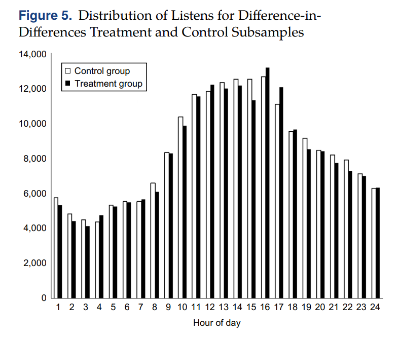
• 2) 노래가 Posting 되는 time 은 exogeneous 하다. The hype machine 에 의해서 결정되는 것이 아니라 Original MP3 blog (여러 음악과 관련된 블로그들) 들을 통해 posting 된다.
• 3) 장르나 인기도 관점에서 각 그룹의 song 들의 특성이 비슷하다. 또한 분석에서 sample 들 간의 유사성을 높이기 위해 CEM 매칭 방법을 적용한다.
• 4) DiD 의 필수적인 가정인 Common trend 를 만족하고 있다.
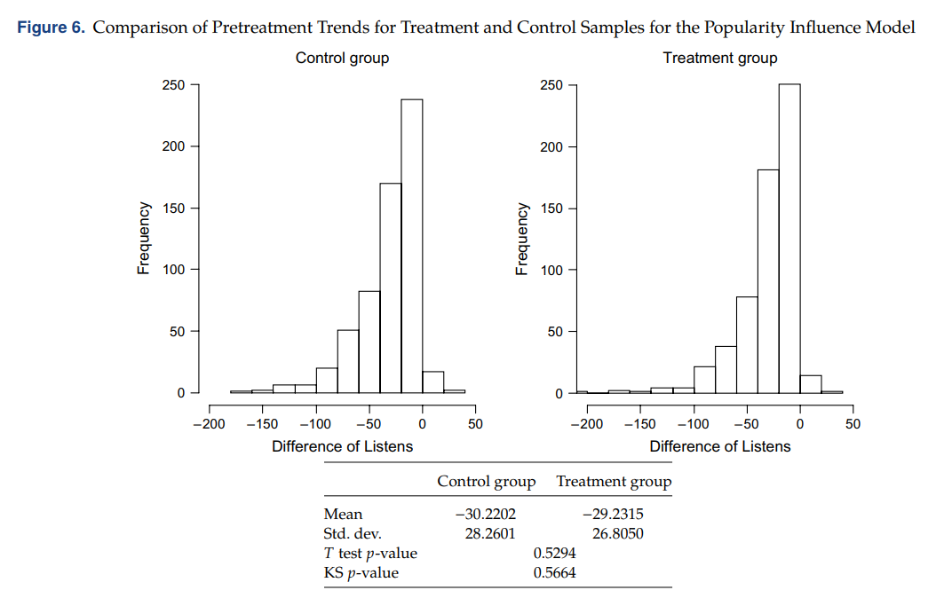
| Treatment and control groups have a common trend in the absence of treatment =assumption of a common pretreatment trend for the treatment and control samples
음악청취 횟수가 시간이 지남에 따라 감소하는 경향을 보이는데, 노래마다 포스팅 시간이 다르므로, 처치집단과 통제집단 간 pretreatment trend 를 비교하기 위해, posting 이후의 처음 12시간 window 와 두번째 12시간 window 각각의 평균적인 청취 수의 차이 (Difference of Listens) 를 사용했다. (시간이 지남에 따라 청취 수는 감소하는 경향을 보이므로 Difference of Listens 가 대부분 음수값을 가짐) 이때 두 그룹 간 분포가 유사하고, t-test 결과도 mean difference 가 insignificant 한 결론을 내렸기 때문에 가정을 만족한다고 볼 수 있다.
• 5) Robustness check : 데이터를 수집한 기준 시점 (9/29,22 말고) 을 달리 하면서 분석을 진행함 → Not sensitive to exactly when the songs are posted
▢ Model specification
↪ song j on day t : 분석 단위는 Song level
↪ t = {T0-1, T0+1, T1-1, T1+1}
↪ PopTreatment_j : 1이면 treated group, 0이면 control group
↪ After_t : 1이면 post-treatment, 0이면 pre-treatment period
↪ β4 : PopTreatment_j X After_t : magnitude of popularity influence ⭐
⑵ Proximity influence
▢ 기본 가정
• Assumption: 주변 친구가 특정 song 에 좋아요를 누른 행동이, 유저가 해당 song 을 듣는 것에 미치는 영향 : How favoriting a song by a focal user impacts the listening behavior of her social ties
• User-song 단위 분석
• Treatment group : 해당 노래를 좋아요 누른 친구가 적어도 1명 이상 있는 유저들로 구성
• Control group : 해당 노래를 좋아요 누른 친구가 단 한명도 없는 유저들로 구성
▢ Propensity score matching
• Control for potential homophily
• 매칭 단위 : User 를 기준으로 매칭 (e.g. User A - User B)
• 매칭 목표 : Control group 의 유저들을 음악취향, 유저에 대한 관측 가능한 특징, 친구 수를 기준으로 Treatment group 에서 가장 유사한 유저와 매칭시키는 것이 목표 → 유저에 대한 demographic 한 정보가 없기 때문에 추천 시스템과 비슷하게 song listening behavior 를 기반으로 매칭을 진행함
• 매칭 기준 : Relative song listening profiles of users (taste)
↪ 유저의 청취 기록 데이터를 기반으로 하여, 3주 기간동안 각 유저에 대해 profile 을 생성하는 것이 목표
↪ 약 8만개의 노래에 대해 장르, 아티스트 인기도 등 다양한 데이터들을 수집해 노래에 대한 정보를 보완한다.
↪ 각 User-Song pair 에 대해, 유저가 특정 노래를 들은 횟수를 기준으로 하여 해당 유저에 대한 전체 청취 횟수의 백분율로 Weight 를 계산하였다. 그런 다음 유저가 청취한 모든 노래를 기반으로 28개의 가중평균된 노래 특성을 반영한 하나의 벡터로 만들었다. 이 결과를 통해 유저의 Profile 을 일련의 숫자 (노래 특성의 가중 평균)로 요약할 수 있으며, 각 숫자는 특정 음악 특성에 대한 사용자의 취향을 나타낸다.
↪ 생성된 Profile 은 PSM 에서 두 그룹의 유저를 매칭시키기 위해 사용된다.
↪ 두 그룹에 속한 각 Song 에 대해서, 유저의 청취기록, 친구 수, 특성을 반영한 logit model 을 기반으로 Treatment group 에 속할 확률을 할당한다.
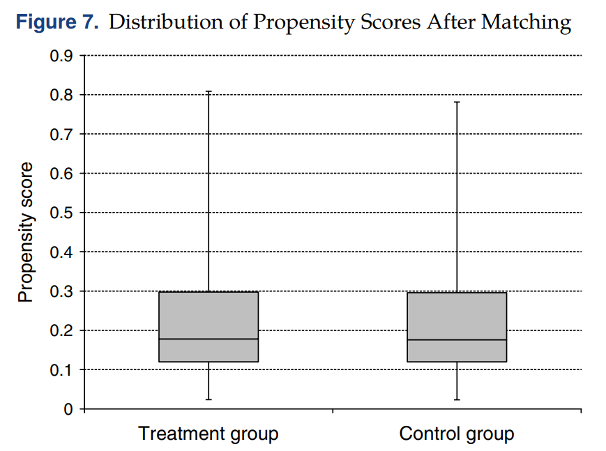
• Propensity score 0.1 이내에 있는 관측치들을 기준으로 매칭 (Caliper = 0.1)
• PSM 이후에 각 그룹의 Propensity score 분포를 나타내 유사도를 확인
※ 보충 설명
• Ti : 처치집단에 있는 User : Song j 를 들어본 적은 없지만 팔로잉한 친구가 좋아요를 누른 경우에 속한 집단의 User
• Ci : 통제집단에 있는 User : Ti 의 유저와 비슷한 taste 를 가지고 (based on listen profile), song j 를 들어본 적이 없으며 해당 노래에 좋아요를 누른 친구가 한 명도 없는 경우에 속한 집단의 user
0. 3주 기간동안의 유저의 listening behavior 를 profile 함 (28개의 음악 특성을 포함하는 vector 와 팔로잉 수를 기준으로)
1. Treatment group (T) 을 정의 (Ti 설명 참고)
2. Potential control group PC 를 정의 : T 에 속하지 않는 user
3. Control group (C) 를 정의한다. 유저의 taste profile 에 기반하여, treated 받을 propensity 를 예측하는 logit model 을 활용해, 주어진 song 을 청취할 Propensity 를 매칭 (Matching the propensity of listening to any given song) 한다. T에 속한 각 user Ti 를 PC 에 속한 PCi 유저와 매칭하고, 매칭된 유저들을 group C 로 정의한다.
4. T와 C 에서 user-song observation 들을 복구 (Recover) 한다. 각 song j 에 대해 만약 user Ti 가 song j 를 좋아요 누른 친구가 있다면 user-song j pair 를 재구성한다. 이후 song j 에 좋아요를 누른 친구가 없는 user Ci 와 매칭을 진행한다.
▢ Euclidean Distance Matching
• Robustness check 을 위해 사용
• 매칭 단위 : User-song level → 각 song 에 대해 > 각 user 를 매칭 : 유저가 주어진 노래를 청취할 likelihood 뿐만 아니라 해당 노래를 좋아하는 친구를 가질 likelihood (the likelihood of being treated) 까지 고려하여 매칭을 진행한다.
• 매칭 기준 : 해당 노래를 들어본적은 없으나 좋아요를 누른 친구가 있는 유저 Ti 와, (Ti와 비슷한 노래 취향을 가지고, 해당 노래를 들어본 적이 없고, 그러나 해당 노래를 좋아할 가능성이 높은 (아직 좋아요를 누른 것은 아님) 친구를 가진) 유저 Ci 와 매칭을 진행한다. 238 개의 treatment user-song pair 가 있다. 이처럼 user-song level 로 분석하면 treated observation 개수가 매우 적어지는데, 이런 경우 로지스틱 회귀분석을 적용하게 되면 다루기 어려워진다. 이를 완화시키기 위해 매칭 과정에서 유클리디안 거리를 사용한다.
※ 보충 설명
0. PSM 과정과 동일하게 user 의 청취행동에 대한 Profile vector 를 생성하고
1. 각 song j 에 대해
∘ 1-(a). Tj (treatment group) 을 결정한다 : song j 를 들어본적은 없지만 좋아요를 누른 친구가 있는 유저
∘ 1-(b). PCj (potential control group) 을 결정한다 : song j 를 들어본적이 없고, 해당 노래에 좋아요를 누른 친구도 없는 유저
∘ 1-(c). 0번째 단계에서 구한 벡터 값을 기반으로 Tj 와 PCj 에 있는 유저들 간의 유클리디안 거리를 계산한다. Treatment group 에 속한 각 유저에 대해, 유클리디안 거리가 가장 짧은 PC group 에 속한 3명의 candidate 유저들을 선택한다.
∘ 1-(d). Cj 를 결정한다 : 1-c 에서 정한 candidate user 들의 각 profile 과 song j 의 profile 의 유클리디안 거리를 비교하여 가장 짧은 거리를 가지는 user 를 선택한다.
∘ 1-(e). Recover user-song j pair for users in Tj, Cj
▢ Probit model
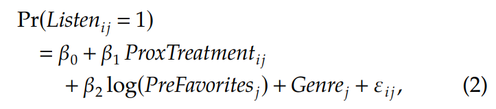
• Examine the impact of proximity influence on the likelihood of listening to a song → implement a binary probit model (해당 노래를 듣게 될 확률을 예측)
• 9월 22일에 posting 된 노래를 대상으로, 노래가 posting 된 이후 48시간 동안 burn-in period 를 allow 하여 favorites 를 얻을 수 있게 함. burn-in 기간 이후에 유저의 listening choice 를 7일간 following 함
• β1 : coefficient of interest on a focal user’s listen decision, captures the impact of proximity influence on a focal user’s listen decision
▢ Hazard model (Weibull model)
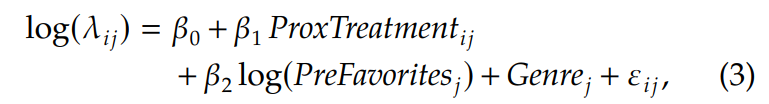
• proximity influence by looking at the time to a user’s first listen to a song
• Hazard model 을 사용하여 user i 가 song j 를 처음으로 듣기 전 기간에 proximity influence 가 끼친 영향에 대해 추정
• hazard rate : λ_ij → defined by whether and when user i listened to song j
• β1 : coefficient of interest
⑶ Combined
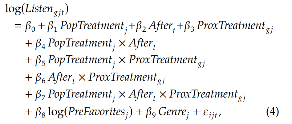
• 두 영향을 동시에 고려한 DDD 모형 : popularity treatment + After_t + proximity influence treatment
• Song j 는 DD 분석과 동일하게 data set 을 설정
• 이후 PSM 을 통해 두 Proximity group 에 속한 유저들을 매칭함
• Listen_gjt : total number of listens of proximity treatment type g of song j at time t , where t = {T0-1, T0+1, T1-1, T1+1} ⁂ song j 의 총 청취횟수
• After_t : pretreatment or posttreatment for popularity
• β3 : represents the magnitude of proximity influence
• β5 : represents the magnitude of popularity impact
• β7 : three-way interaction term : nature of interaction between popularity and proximity influence (β7 > 0 : complementary, β7 < 0 : substitute)
⑤ Results
◯ Popularity influence
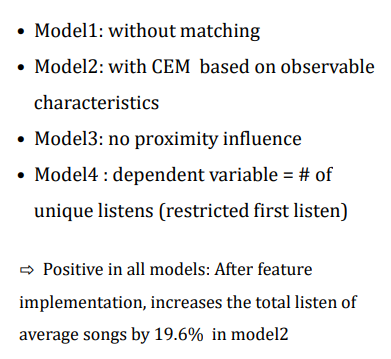
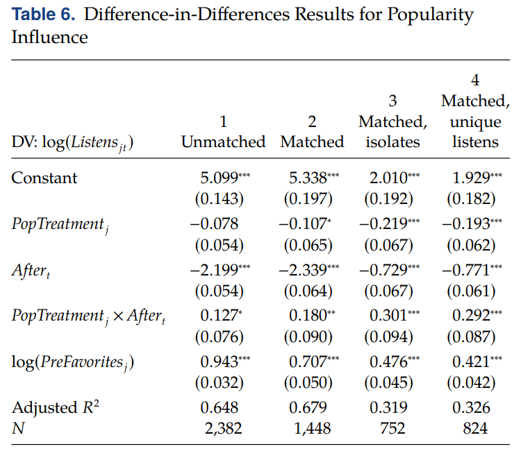
▢ 해석
• (Matching 후) N 에 주목하기
• PopTreatment x After : captures the average effect of the treatment on the number of listens after the availability of song popularity information on the website (노래 인기 정보 공개와 사용자 청취 횟수 사이의 인과관계)
• After feature implementation, increases the total listens of average song by 19.6% (exp(0.18)) in model2
• magnitude and significance are highest in model 3 and 4 = Popularity influence is strongest for isolates (users with no friends) and for the first listen of a song (↔ repeat listens)
▢ Robustness check
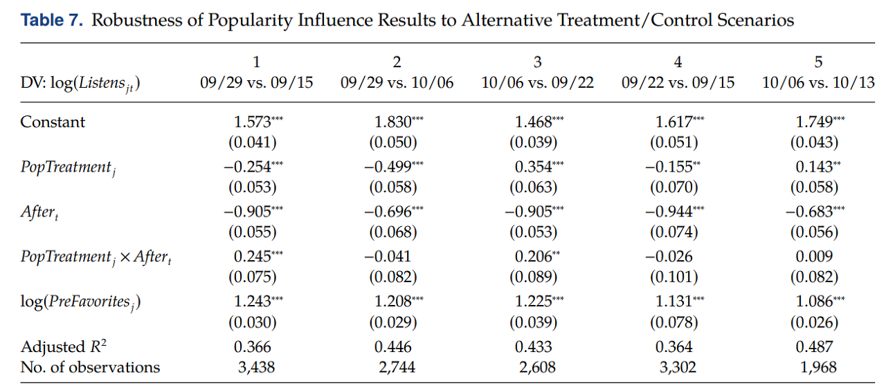
• Validating DD research design with the treatment and control samples drawn from neighboring weeks
• 특정한 요일을 선택했기 때문에 나타난 결과가 아님을 (for generalize) 밝히기 위해 다른 대안적인 요인들을 선택해서 모델링을 진행 ⇒ Robust and there no “secular” effects in different weeks
▢ Narrow-appeal music VS broad appeal music
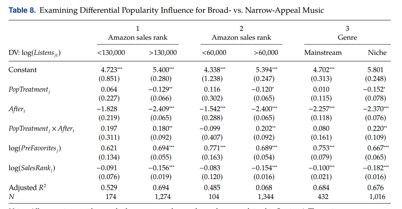
• 아마존 음반 판매 순위 및 주류/비주류 장르를 기준으로 Song group 을 구분
• 세 모델에서 모두 interaction term 의 계수에서 positive in sign, but significant only for narrow appeal song samples
◯ Proximity influence
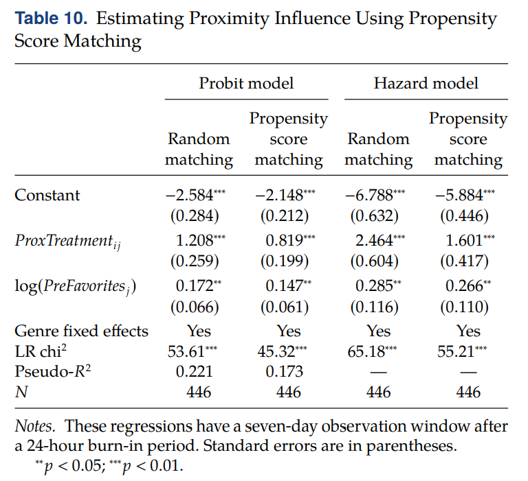
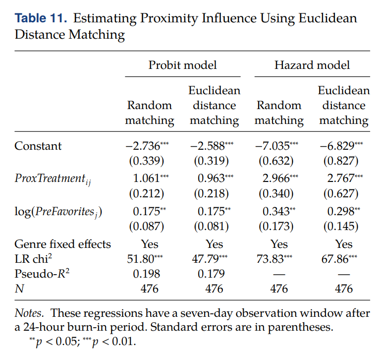
• ProxTreatment → probit, hazard 모델에서 모두 positive & significant 하고, random matching 보다 PSM or EDM 일 때 magnitude of coefficient 가 goes down 함 (to be able to isolate it from homophily)
◯ Combined model of Popularity and Proximity influence
• user-song granularity : Listen_gjt ⇒ g : user proximity group, j : song, time t
🤔 논문에서 dependent variable 을 log(Listen_git) 로 설정하고, Treatment 와 Control group 을 PSM 매칭하는 과정에 대해 추가적인 설명이 없음 (Supplement 자료도 없음)
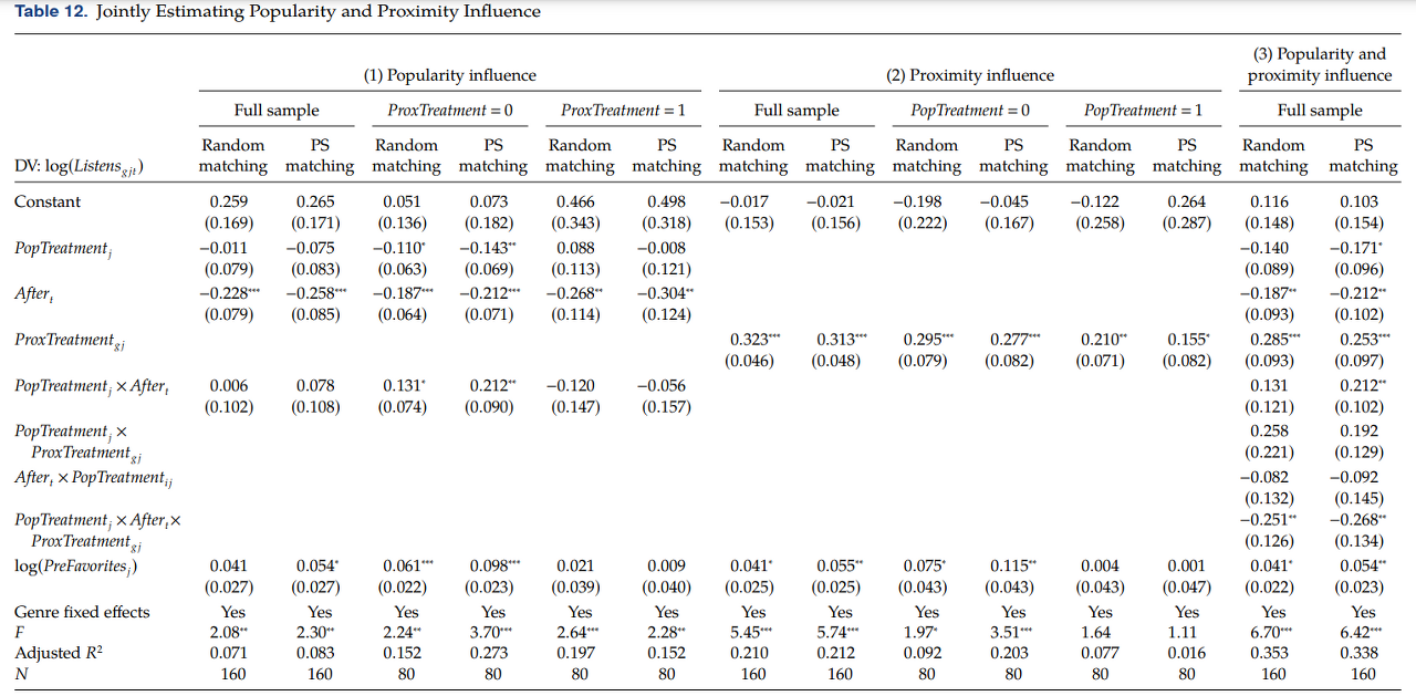
• Model1. Populairty influence
↪ PopTreatment x After
∘ Full sample 일 땐 not significant ⇨ due to sparseness of total listens at the user-song granularity : User-song 단위로 matching 된 데이터셋으로 진행되었기 때문 (N=160) ⇨ g index (기간 T0, T1 에 속하는 Song j 에 대해, Proximity 조건에 맞는 user 들을 추리다 보니 N의 개수가 매우 줄어듦)
∘ subsample analysis 에서 ProxTreatment = 0 일 때만 (=user does not have a friend who has previously favorited the song) PSM 에서 계수가 significant 함 ⇒ substitutes 관계
• Model2. Proximity influence
↪ PopTreatment_gj
∘ full model → positive and significant & magnitude declines under PSM
∘ subsample analysis 에서 PopTreatment 가 0일 때 (absence 할 때) ProxTreatment 변수가 greater sign and significance 한 것으로 나타났다 ⇒ substitutes 관계
• Model3. Popularity & Proximity influence
↪ PopTreatment_j x After_t x ProxTreatment_gj
∘ coefficient is negative and significant → popularity and proximity influence are substitutes
∘ specifically, popularity influence is less important in the presence of proximity influence
⑥ Conclusion
'3️⃣ Study at Univ > ○ 논문읽기' 카테고리의 다른 글
| [Causal Forest] 머신러닝 기반의 인과 포레스트 기법을 활용한 처치효과 검증: 교내 동아리활동 참여가 협업능력에 미치는 효과를 중심으로 (1) | 2024.01.23 |
|---|---|
| Graph Clustering with Graph Neural Networks (2020) (1) | 2022.12.23 |
| DeepWalk (1) | 2022.11.03 |
| 앱 리뷰 분석에 관한 논문 정리 ③ (0) | 2022.06.16 |
| 앱 리뷰 분석에 관한 논문 정리 ② (0) | 2022.06.15 |


댓글