인과추론의 데이터 과학 - 가상의 통제집단
참고영상 : Bootcamp 3-4. 가상의 통제집단
1. synthetic control vs DID
◯ Synthetic control
• synthetic control 은 DID 의 확장버전이나 좀 더 유연한 방법이다.
• 매칭이 성립되지 않고, parallel trend 가정이 성립하지 않더라도 적용할 수 있다.
• 최근 가장 주목받는 방법론이기도 하다.

• control group 을 조합함으로서 가상의 비교가능한 통제집단을 구성할 수 있는 방법이다.

2. Example
◯ 캘리포니아의 담배 규제의 담배 판매량에 미친 효과

• 캘리포니아에서만 1988년에 도입됨, 규제가 도입되지 않은 49개의 다른 주와 비교하고자 하지만, 위의 그림과 같이 parallel trend 를 따르지 않음 ⇨ synthetic control 이 필요

• synthetic 캘리포니아를 만들기 위해, 각 주에 대해 weight linear combination 을 통해 캘리포니아를 모방할 수 있는 가상의 주를 만든다.
• Donor pool : synthetic control 을 만드는데 투입되는 control unit
◯ 서독과 동독의 통일이 경제에 미친 인과적 효과
• 통일이 되지 않았더라면 있었을 counterfactual 자체는 관찰할 수 없음
• 독일과 유사한 상황의 국가를 찾기도 어려움
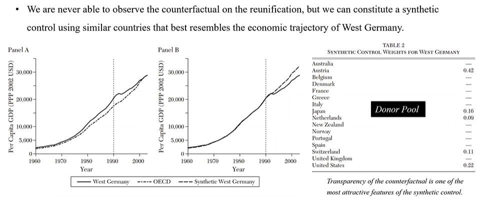
• Synthetic control 을 적용하여, 주변 국가들을 적절히 weight 을 주어서 조합했더니, 서독의 경제를 모방하는 가상의 국가를 만들 수 있었다.
• Donor pool 에서 weight 을 어떻게 설정하느냐가 관건
3. How to construct the synthetic control
◯ Original Method

• treatment 를 받기 이전의 outcome 과 predictor 에 대해서 처치그룹에서의 값과 통제집단에서의 조합에서의 차이가 최소화 되도록 rate 을 구한다.
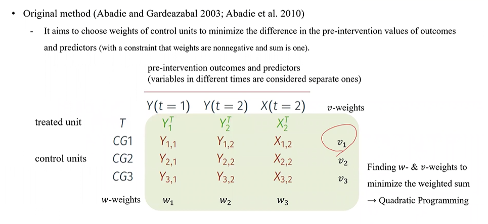
• control unit 에서의 조합으로 treated unit 에 가까워질 수 있는 weight 을 찾기 ⇨ optimization 문제
• t=1 인 시점의 outcome, t=2 인 시점의 outcome, t=2 인 시점에서의 predictor X ⇨ 세 변수들 간의 weight 을 고려 : w-weights
• control unit 별로 어떻게 weight 을 주어서 synthetic control 을 만들지 : v-weights
⇨ W1∙(Y1' - (V1∙Y1,1 + V2∙Y2,1 + V3∙Y3,1)) + W2∙(Y2' - .....) + W3∙(Y3' - .....) 를 minimize 하는 weight 찾기
⇨ W, V의 이차항 문제 : Quadratic programming
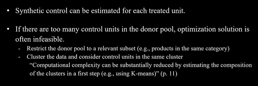
• synthetic control 은 각각의 treated unit 에 대해 따로 구할 수 밖에 없다.
• optimization 문제이기 때문에 control variable 이 많으면 시간이 오래걸리고 최적값이 도출되지 않을 수 있다. 모든 control variable 이 모두 donor pool 이지 않아도 된다. donor pool 을 적절히 줄이는 것도 중요하다.
◯ Various methods

• negative weight 을 쓰거나, 엘라스틱넷/라쏘 등을 사용하거나 다양한 방법들이 생겨나고 있다.
◯ Synthetic difference in difference

• 기존의 synthetic control 은 시간에 따른 변화를 크게 고려하지 않고, control unit 과 변수에 대한 weight 만을 고려한다. 그러나, synthetic DID 는 기존의 DID 처럼 unit fixed effect 와 time fixed effect 를 모두 고려하고, 동시에 기존의 synthetic control 처럼 동작하면서, time weight 도 고려한다. 이를통해 fixed effect 와 weight 을 모두 고려할 수 있게 된다.
◯ Bayesian synthetic control


• synthetic control 은 prediction problem 으로 귀결될 수 있다. out of sample prediction 문제이기 때문에 머신러닝 방법론이 많이 적용되는 분야이다.
4. Inference for synthetic control
◯ Placebo test
• 통계적으로 synthetic theory 에 기반에 standard error 나 p-value 를 구할 수가 없다.
• synthetic control 을 할 때, 어떠한 식으로 inference 를 하냐 ⇨ Placebo test : synthetic control 과 actual 값의 차이가 treatment 전후로 얼마나 차이가 나는지 확인한다.

• treatment 이후에 실제값과 synthetic control 간의 차이가 100배 이상으로 큼
• 옅은 회색 선들은 캘리포니아를 제외한 나머지 주들에 대한 synthetic control 과 실제 값의 차이
• 다른 대부분의 주들에서는 treatment 이전과 이후에 차이가 별로 없다 (실제 treatment 가 없었기 때문) ⇨ 캘리포니아에 대한 효과가 유의하다고 결론내릴 수 있다.
5. Sensitivity tests for synthetic control

• synthetic control 을 어떤 변수로 구성하는지에 따라 달라짐 : variable (predictors) 에 대한 sensitivity test 가 필요
• donor pool 내에서 control unit 에 대한 weight 에 대해서도 sensitivity test 가 필요
• 여러가지 가능성에 대해 robust 한 경우의 수를 찾기

• prediction 문제이기 때문에 머신러닝에서 적용하는 Train , test 데이터 split 도 synthetic control 에 적용해볼 수 있다.
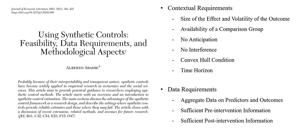
6. Requirements for synthetic control
• 더 공부해보고 싶다면 review paper 살펴보기!
👀 Control group 이 없다면 → Time series forecasting model can be used to predict the counterfactual, 그러나 이러한 경우 외부 충격 이후에 대한 예측은 다소 어려울 수 있음