데이터마이닝 Preprocessing ②
1. Types of data sets

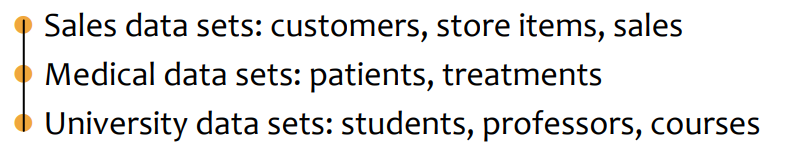
• Relational Records
↪ collections of records, each of which consists of a fixed set of attributes

• Data matrix: record data
↪ If the data objects have the same fixed set of numeric attributes, the data objects can be thought of as points in a multi-dimensional space, where each dimension represents a distinct attribute
↪ m by n matrix, m rows, n columns

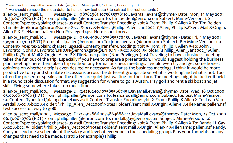
• Document data: record data
↪ Each document becomes a term vector (word vector)
↪ Each term is a component of the vector
↪ The value of each component is the # of times the corresponding term occurs in the document

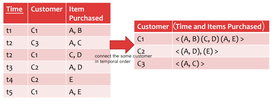
• Transaction data: record data
↪ special type of record data, where each record involves a set of items
↪ Also called market basket data

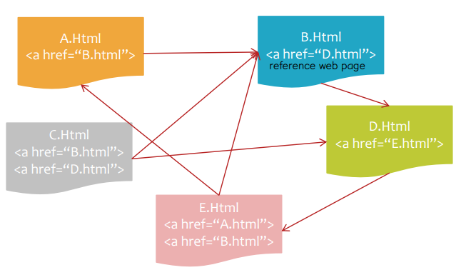
• WWW data: graph data
↪ world wide web: HTML links between web pages can be represented as a graph
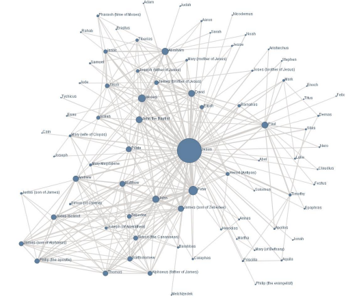
• Social network data: graph data
↪ Relationships (friends, followers) between users can be modeled as a graph
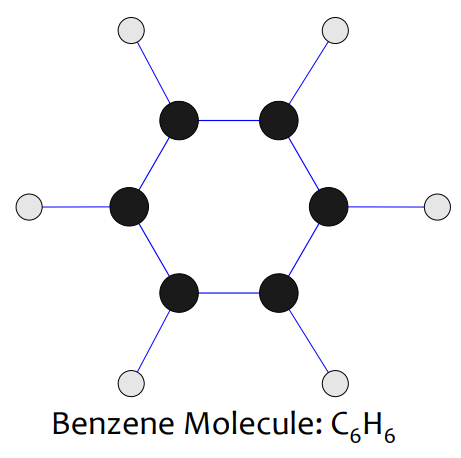
• Molecular structures: graph data
↪ Chemical compounds originally have the graph structure
• Sequential data: ordered data
↪ Sequences of transaction
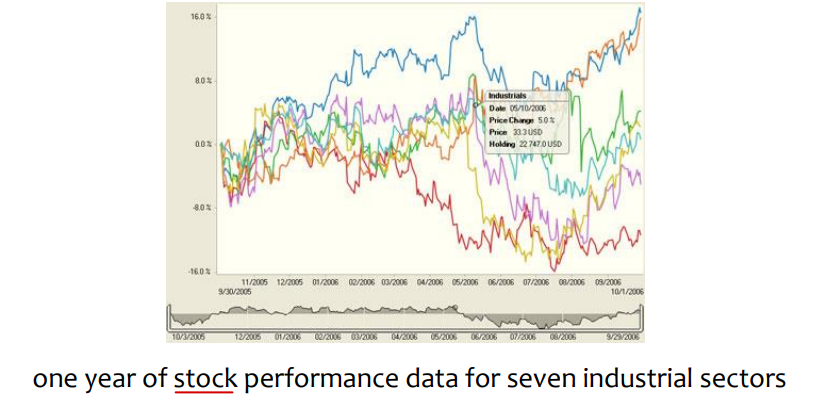
• Time series data: ordered data
↪ Sequences of data points, measured typically at successive items spaced at uniform time intervals
(일, 월, 연도)
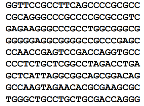
• Genetic Sequence data: ordered data
↪ Nucleic acids consist of a chain of linked units called nucleotides
• Trajectory data: ordered data
↪ Sequences of the locations and timestamps of moving objects → Usually represented by latitude and longitude

• Text data: ordered data
2. Data objects and attribute types
• Data objects
↪ data set can often be viewed as a collection of data objects
↪ data object (or sample, example, instance, point, tuple) represents an entry
↪ data objects are described by attributes
↪ In relational databases, rows are data objects, columns are attributes
• Attributes
↪ attribute (or dimension, feature) is a property or characteristic of an object
↪ Types
▸ categorical : qualitative → Nominal, Ordinal
▸ Numeric : quantitative → Interval, Ratio
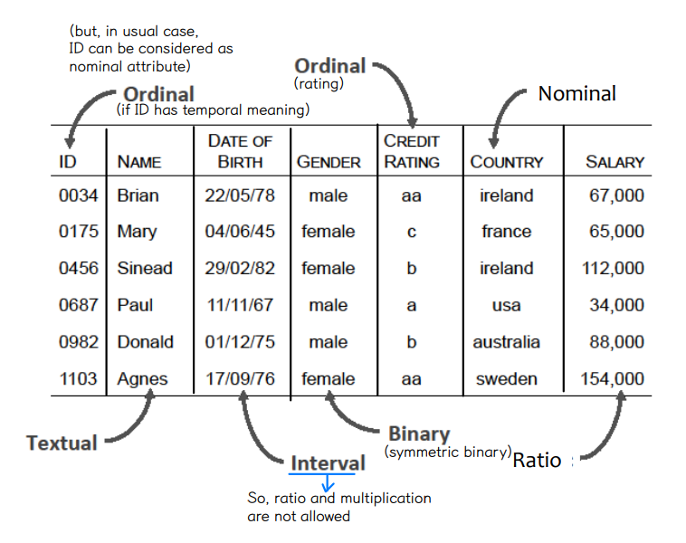
① Categorical attributes types
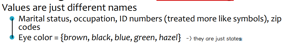
1) Nominal : categories, states, or "names of things"
2) Binary : special type of nominal attribute
▸ Nominaattributete with only 2 states (0,1)
▸ Symmetric binary : both outcomes s equally important
⇨ ex. female and male
▸ Asymmetric binary : outcomes not equally important
⇨ ex. medical test (positive vs negative : positive is more important
▸ Convention : assigning to 1 most important outcome
⇨ ex. HIV positive
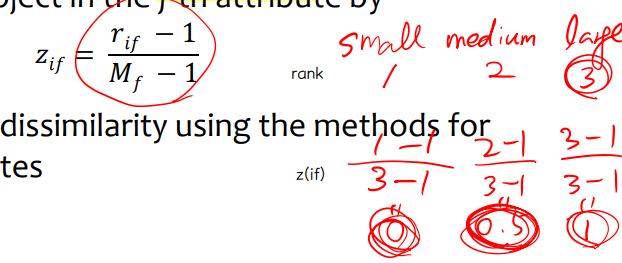
3) Ordinal : values have a meaningful order (ranking), but the magnitude between successive values is not known
▸ Ex. Sizes (={small, medium, large}), grades, army rankings
▸ CQA ) the median of even-numbered ordinal dataset cannot be accurately calculated, but ex, 9 shirts can have sizes from {XXS, XS, S, M, L, XL} in ascending order as follows : XXS, XS, S, S, M, M, L, XL. Then the median is clearly S.
▸ CQA ) we do not define the order for any set of attributes. For example, the lexicographic order for names is just for convenience.
② Numeric attribute types
1) Interval
▸ Values are measured on a scale of equal-sized units: values have order
⇨ ex . temperature in C∘ or F∘, calendar dates
▸ No true zero-point
⇨ ex. 0C∘ is in a physical sense, arbitrary (cf. 0K∘) ⇨ In a physical sense, zero celsius is arbitrary
2) Ratio
▸ Inherent zero point (true zero point)
▸ We can speak of values as being an order of magnitude larger than the units of measurement
⇨ ex. 10K∘ is twice as high as 5K∘
⇨ ex. temperature in Kelvin, length, counts, monetary quantities
③ Possible data analysis
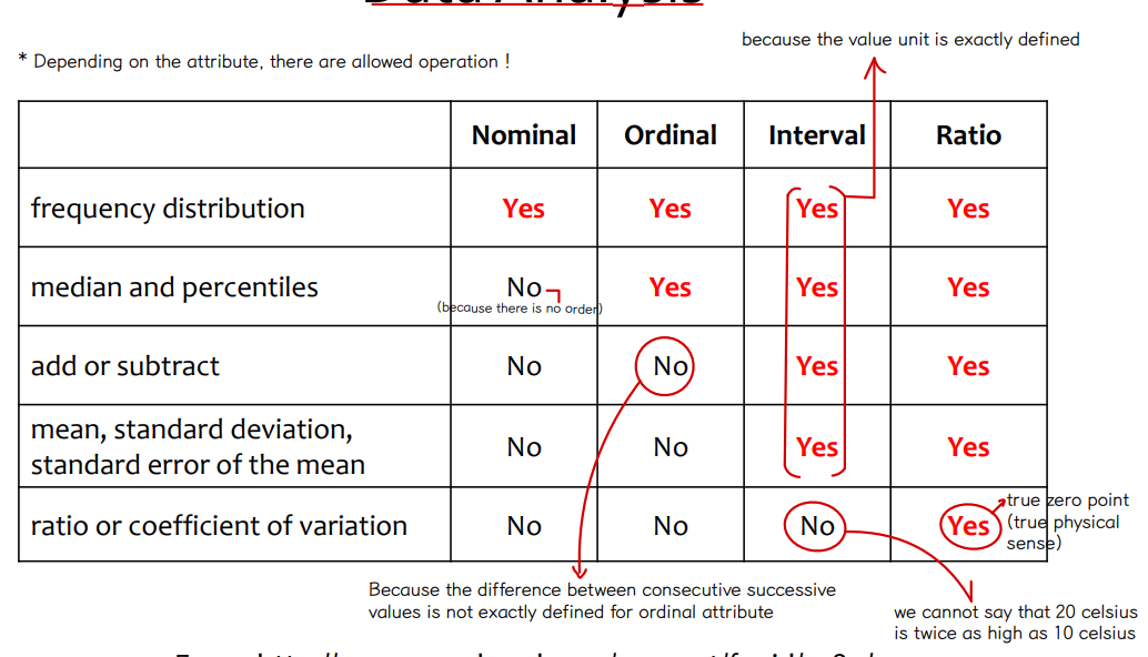
⇨ Ordinal attributes 는 중앙값, percentile 을 계산할 수 있다. (CQA 참고)
⇨ interval attributes 는 ratio 나 coefficient of variation 을 계산할 수 없다.
• Continuous vs Discrete Attributes
↪ Discrete attribute: A finite number of possible values, can be represented as integer variables
↪ Continuous attribute: infinite number (ex. temperature, height, weight), Typically represented as floating-point variables
3. Basic statistical description of data
• Central tendency
↪ Mean
↪ Median : The middle value of the ordered set if the number of data is odd; otherwise, the average of the two middle values (데이터가 홀수개면 가운데 값, 짝수개면 중간에 있는 두 값의 평균값)
↪ Mode : The value that occurs most frequently in the set
⇨ Unimodal : only one mode
⇨ Bimodal : two modes
⇨ Multimodal : multiple modes
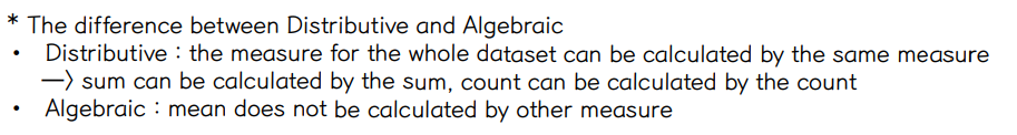
• Types of Measures
↪ Distributive: A measure that can be computed for a given data set by partitioning the data into smaller subsets, computing the measure for each subset, and then merging the results in order to arrive at the measure’s value for the original (entire) data set
⇨ ex. sum, count, min, max
↪ Algebraic: A measure that can be computed by applying an algebraic function to one or more distributive measures.
⇨ ex. mean = sum/count
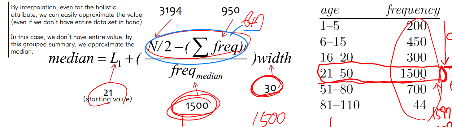
↪ Holistic: A measure that must be computed on the entire data set as a whole
⇨ ex. median → exact value for the whole dataset,cannot be calculated by each subset
• Approximation of the Median
↪ The median value of a data set can be easily approximated by interpolation for grouped data
• Symmetric vs Skewed data
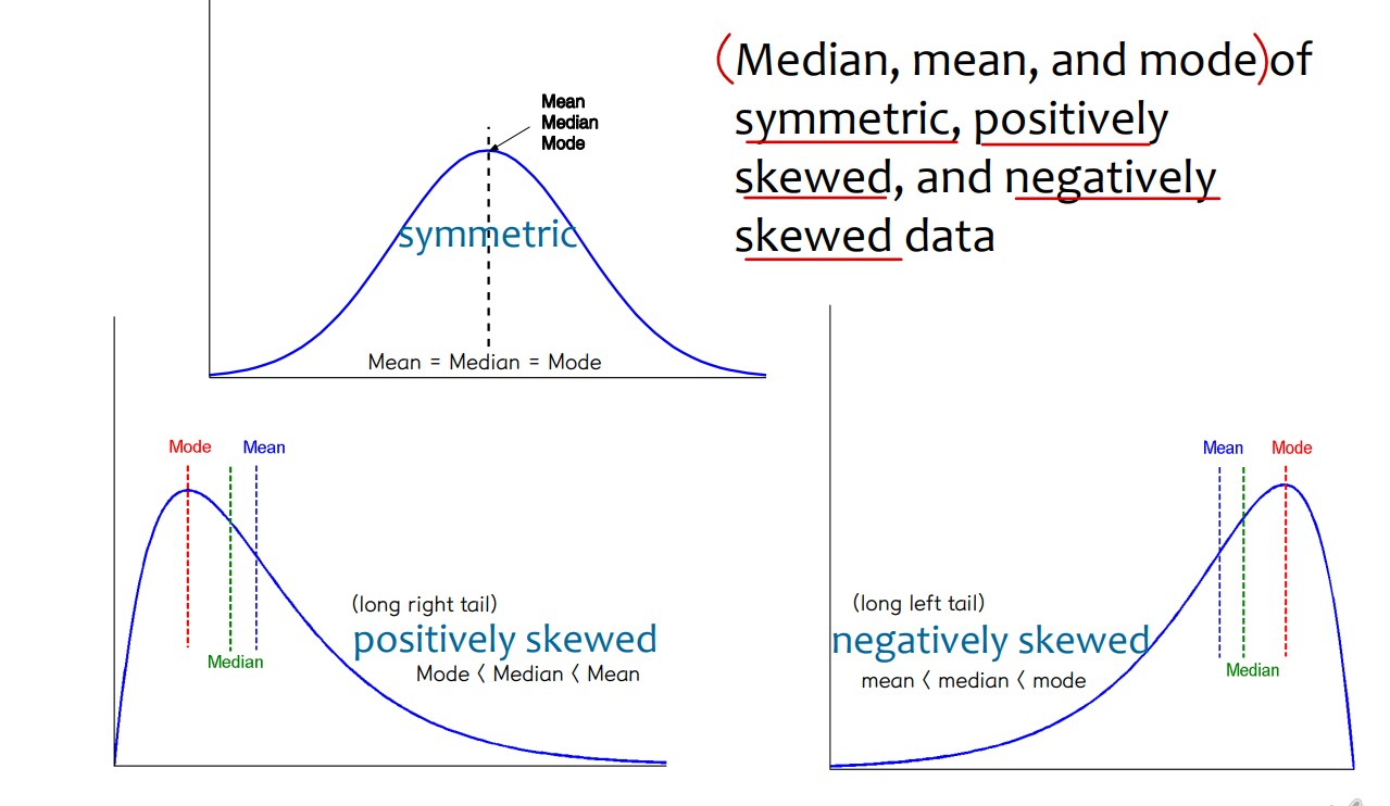
⇨ Positively skewed (long right tail) : mode < median < mean
⇨ Negatively skewed (long left tail) : mean < median < mode
• Dispersion of data
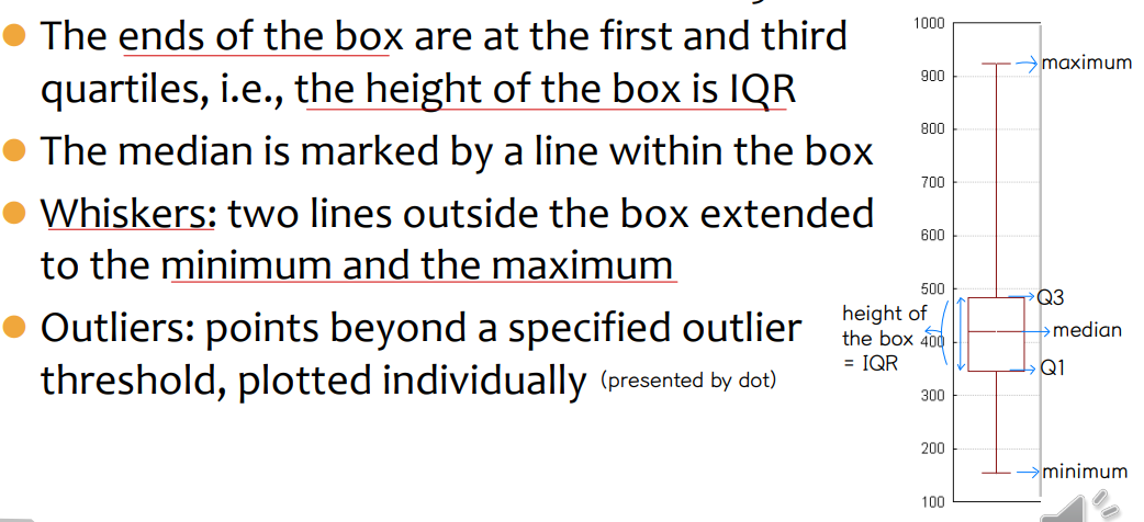
↪ Quartiles
⇨ Q1 (25th percentile) , Q3 (75th percentile), Q2 (median, 50th percentile)
⇨ IQR = Q3 - Q1
⇨ Five number summary : min, Q1,Q2,Q3, max
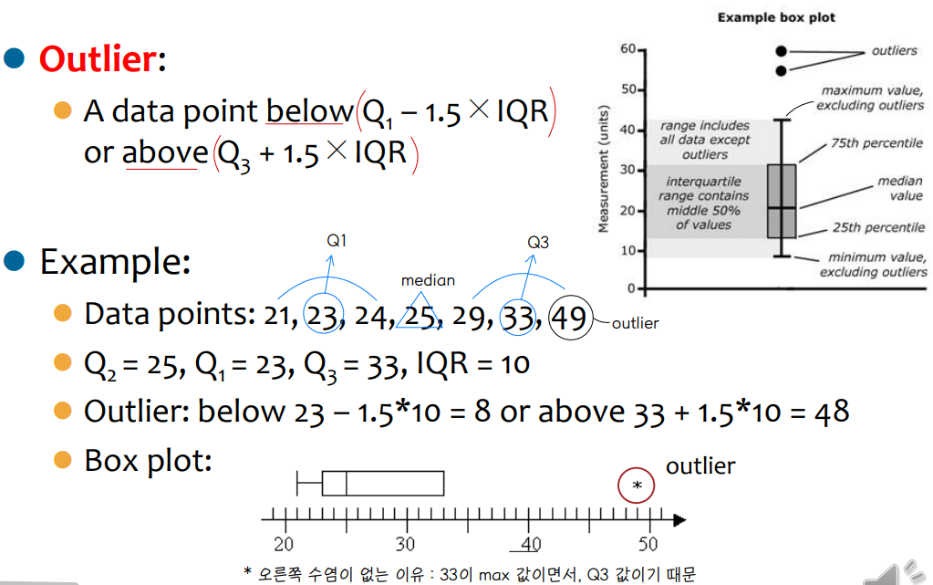
⇨ Outlier : usually , a value higher/lower than 1.5 X IQR
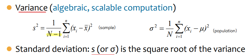
↪ Variance and standard deviation
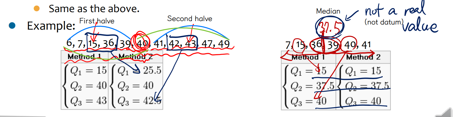
• Quartile 구하는 방법
↪ 첫번째 방법
⇨ 중앙값을 포함하지 않고, 중앙값을 기준으로 절반으로 데이터를 나누어서 계산하는 방법
↪ 두번째 방법
⇨ 데이터가 홀수개여서 중앙값이 데이터 내에서 찾아질 때 (datum 이라 부름) 는 중앙값을 포함시키고 절반으로 나누어 계산한다. 만약, datum 이 아니라면, 첫번째 방식으로 (중앙값을 포함하지 않음) 계산한다.
• Graphic Displays of Basic Statistical Descriptions
① box plot
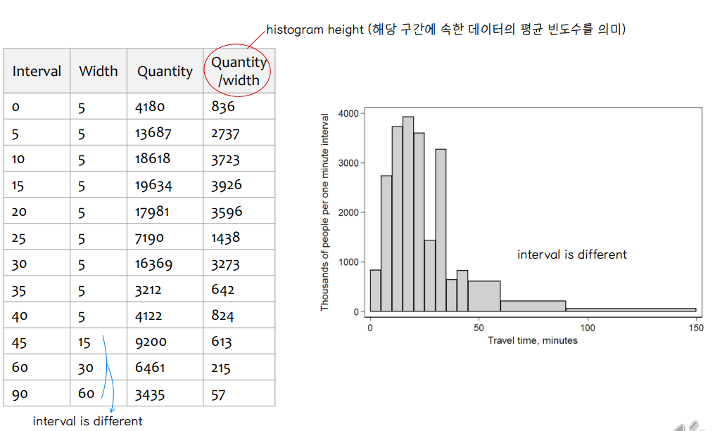
② histogram ⭐
▸ showing a visual impression of the distribution of data
▸ 히스토그램 직사각형 높이 = frequency density of the interval : frequency/width of the interval
▸ The total area is equal to the number of data
③ Quantile plot
▸ For a value xi, when data are sorted in increasing order, fi, indicates that approximately 100 fi % of the data are below or equal to xi
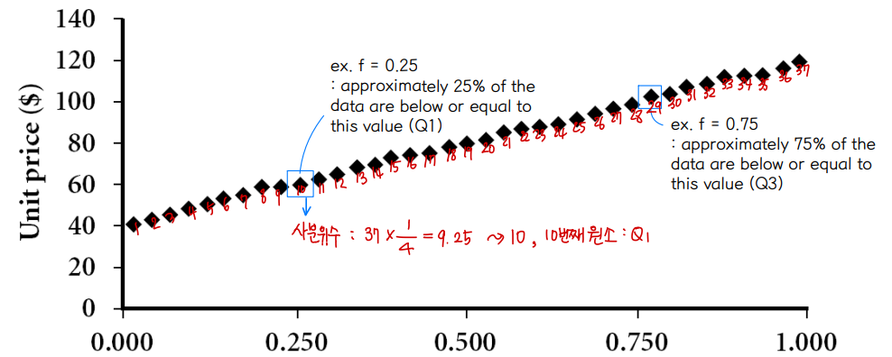
▸ kth q-quantile
⇨ 1 <= k <= (q-1)
⇨ q = 4 : quartile, 1st-4quantile is Q1, 2nd-4quantile is Q2, 1rd-4quantile is Q3
⇨ q = 100 : percentile
④ QQ plot
▸ comparing two probability distributions by plotting their quantiles against each other.
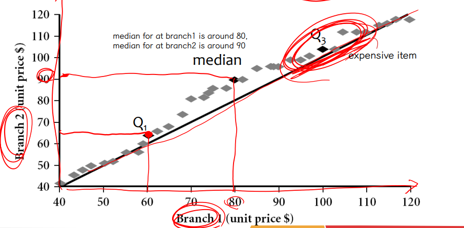
▸ If the two distributions being compared are identical, the Q-Q plot follows the line y = x
⑤ Scatter plot
▸ A type of mathematical diagram using Cartesian coordinates to display values for two variables for a set of data
▸ QQ plot 은 x와 y축에 해당하는 단위값이 동일한 반면 (ex. # of item sold in branch1, # of item sold in branch2) scatter plot 은 단위가 다른 두 변수가 와도 상관 없음
4. Data visualization techniques
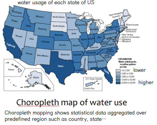
• Thematic Cartography
① Choropleth
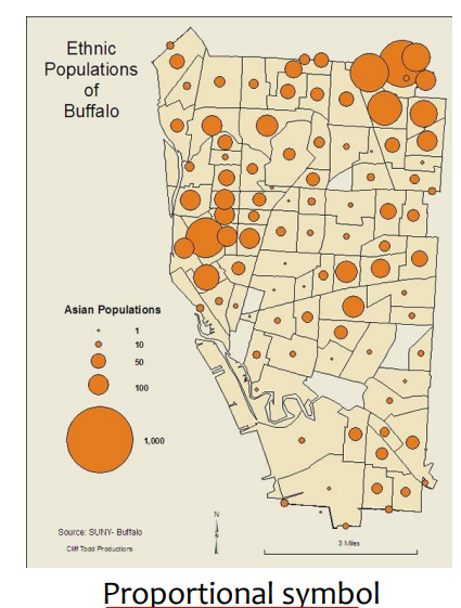
② Proportional symbol
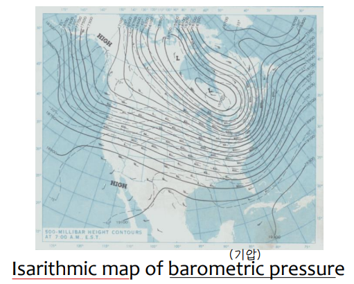
③ Isarithmic
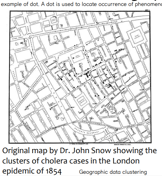
④ Dot
⑤ Dasymetric
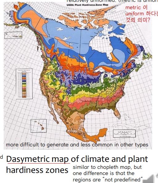
⇨ similar to choropleth map, but one difference is that the regions are “not predefined”
5. Data similarity and dissimilarity
• Dissimilarity between Nominal attributes

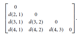
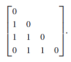
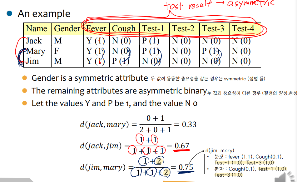
• Dissimilarity between Binary attributes
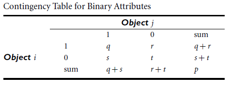
▸ symmetric binary variable
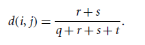
▸ asymmetric binary variable
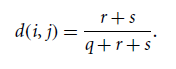
⇨ asymmetric 은 두 개의 상태가 동일한 중요성을 갖고 있지 않기 때문에, 두 값이 모두 negative 한 데이터인 t 는 무시해버린다.
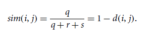
▸ asymmetric binary similarity : Jaccard coefficient
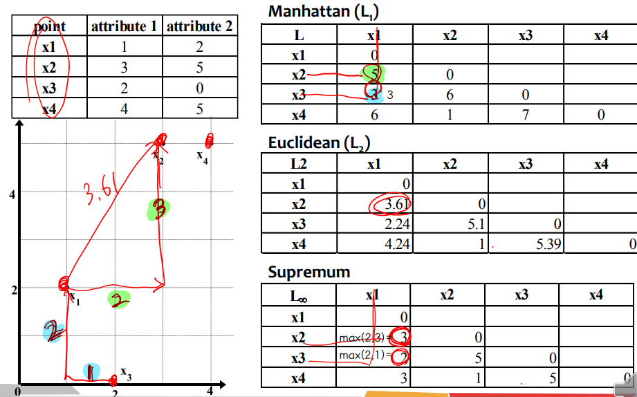
• Distance on Numeric Attributes Minkowski Distance
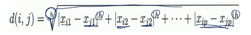
⇨ h = 1 : Manhanttan
⇨ h = 2 : Euclidean
⇨ h → ∞ : supremum
• Common Properties of a Distance
⇨ Positive definities
⇨ Symmetry
⇨ Triangle Inequality
⇨ Dissimilarity
• Dissimilarity between Ordinal attributes
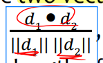
• Cosine similarity
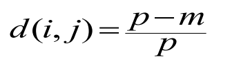
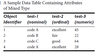
• Mixed types
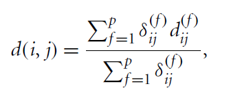
→ 각 타입에 맞는 식으로 게산 후에 다시 통합해준다.

→ 가중치 : weight importance for the f-th attribute